

Mean-field analysis of orientation selectivity in inhibition-dominated networks of spiking neurons
- PMID: 24790806
- PMCID: PMC4003001
- DOI: 10.1186/2193-1801-3-148
Mean-field analysis of orientation selectivity in inhibition-dominated networks of spiking neurons
Abstract
Mechanisms underlying the emergence of orientation selectivity in the primary visual cortex are highly debated. Here we study the contribution of inhibition-dominated random recurrent networks to orientation selectivity, and more generally to sensory processing. By simulating and analyzing large-scale networks of spiking neurons, we investigate tuning amplification and contrast invariance of orientation selectivity in these networks. In particular, we show how selective attenuation of the common mode and amplification of the modulation component take place in these networks. Selective attenuation of the baseline, which is governed by the exceptional eigenvalue of the connectivity matrix, removes the unspecific, redundant signal component and ensures the invariance of selectivity across different contrasts. Selective amplification of modulation, which is governed by the operating regime of the network and depends on the strength of coupling, amplifies the informative signal component and thus increases the signal-to-noise ratio. Here, we perform a mean-field analysis which accounts for this process.
Keywords: Common-mode attenuation; Contrast invariance; Inhibition-dominated; Mean-field analysis; Operating regime; Orientation selectivity; Tuning amplification.
Figures
 , shown for EPSP = 0.1 mV (J = τ
syn
e EPSP = 0.136 mV). For normalization, each entry is divided by the reset potential, V
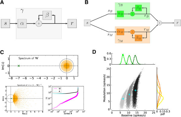
reset = 20 mV. The ‘exceptional eigenvalue’ (green) corresponds to the uniform eigenmode, i.e. the baseline, and the bulk of the spectrum (orange) determines the response of the network to perturbations of a uniform input. Bottom, left: Eigenvalue distribution for the matrix
, shown for EPSP = 0.1 mV (J = τ
syn
e EPSP = 0.136 mV). For normalization, each entry is divided by the reset potential, V
reset = 20 mV. The ‘exceptional eigenvalue’ (green) corresponds to the uniform eigenmode, i.e. the baseline, and the bulk of the spectrum (orange) determines the response of the network to perturbations of a uniform input. Bottom, left: Eigenvalue distribution for the matrix  , which gives the stationary firing rates. Bottom, right: Sorted magnitudes of eigenvalues of
  and
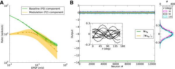
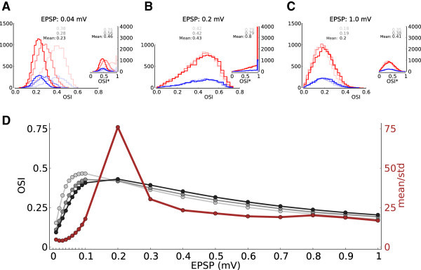
and  . (D) Baseline and modulation components for individual neurons in the network with EPSP=0.1 mV. Scatter plot (center) shows the modulation vs. baseline component of output tuning curves for all neurons of the network. Baseline and modulation are taken as the mean (F0) and the second Fourier component (F2) of individual tuning curves, respectively. The markers (cyan crosses) show the center of mass of each cloud. The histograms indicate the marginal distributions of baseline (green, top) and modulation (orange, right) components, respectively.
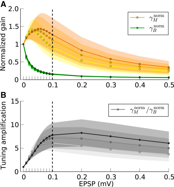
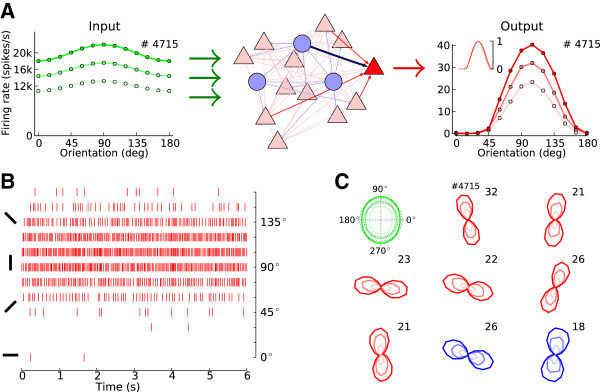
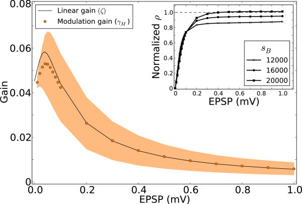
 (green), and modulation gain,
  (orange), for a network with a fixed connectivity, but different strengths of recurrent synaptic couplings. Shaded regions represent mean±std. Lighter colors correspond to lower contrasts. (B) As a result of selective attenuation of the baseline, the normalized modulation-to-baseline ratio (
 ) is generally much larger than 1. The degree of recurrence of the network presented in Figures 1, 2, 3 and 4 is marked by dashed lines.
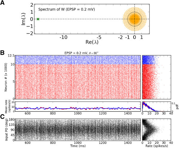
 , shown for EPSP = 0.2 mV (J = 0.27 mV). The same normalization as in Figure 4C is employed, i.e. each entry is divided by the reset potential, V
reset = 20 mV. (B-C) Same plots as in Figure 1A, B, for EPSP=0.2 mV.
, shown for EPSP = 0.2 mV (J = 0.27 mV). The same normalization as in Figure 4C is employed, i.e. each entry is divided by the reset potential, V
reset = 20 mV. (B-C) Same plots as in Figure 1A, B, for EPSP=0.2 mV.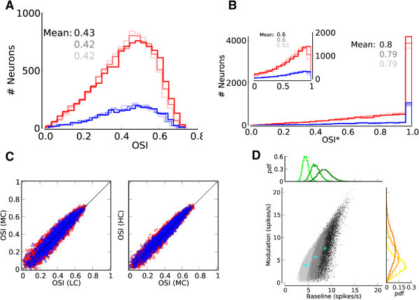
 with a baseline,
  , and a modulation input vector,
  . The entries of the baseline vector are all normalized to one, i.e. the input to each neuron is 1. The operation of the weight matrix on the baseline vector,
  , is plotted in green. The operation of the weight matrix on the modulation vector,
  , for three different orientations (θ = 30°,90°,120°) are plotted in magenta, black and cyan, respectively. The corresponding distributions of individual responses are plotted in the magnified histograms on the right. Note that the assumption of ‘perfect balance’ implies a very narrow distribution around zero. The average (over 12 orientations) of the responses,
  , are plotted in orange. For 12 sample neurons from the network the response vs. orientation of the stimulus are plotted in the inset (center).
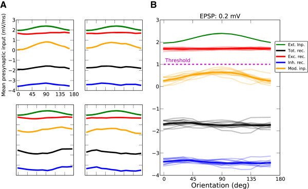
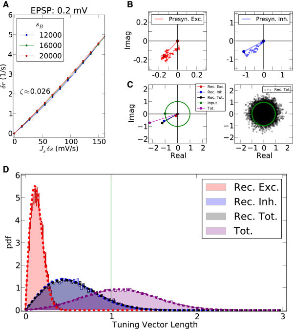
 , weighted by the linear gain (ζ), and vectorially added together, reflecting linear integration in neurons. Although each presynaptic vector makes only a small contribution, the resulting random sum can lead to a large resultant Tuning Vector. These are generally larger for presynaptic inhibition (Presyn. Inh.) compared to presynaptic excitation (Presyn. Exc.). Note different scales of axes. (C) Left panel: The resultant vectors for recurrent excitation (Rec. Exc.), recurrent inhibition (Rec. Inh.), total recurrent (Rec. Tot. = Rec. Exc. + Rec. Inh.), feedforward input (Input), and the total input (Tot. = Input + Rec. Tot.) are plotted. All normalized input Tuning Vectors have the same length of one, denoted by the green circle. Right panel: Total recurrent Tuning Vectors (Rec. Tot.) for all neurons in the network are compared with the normalized length of their input Tuning Vectors (green circle). D) Distribution of the length of all Tuning Vectors for all the neurons in the network. Dashed lines show the predicted distributions of the linear analysis in each case (see text for details).
 .
.References
-
- Alitto HJ, Usrey WM. Influence of contrast on orientation and temporal frequency tuning in ferret primary visual cortex. J Neurophysiol. 2004;91(6):2797–2808. - PubMed
-
- Amit DJ, Brunel N. Model of global spontaneous activity and local structured activity during delay periods in the cerebral cortex. Cerebral Cortex. 1997;7(3):237–252. - PubMed
-
- Anderson JS, Lampl I, Gillespie DC, Ferster D. The Contribution of Noise to Contrast Invariance of Orientation Tuning in Cat Visual Cortex. Science. 2000;290(5498):1968–1972. - PubMed
LinkOut - more resources
Full Text Sources
Other Literature Sources
