Coevolution can reverse predator-prey cycles

Abstract

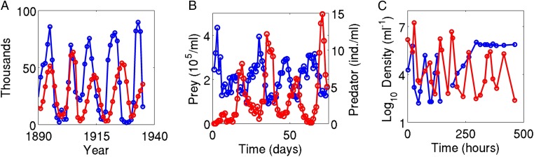
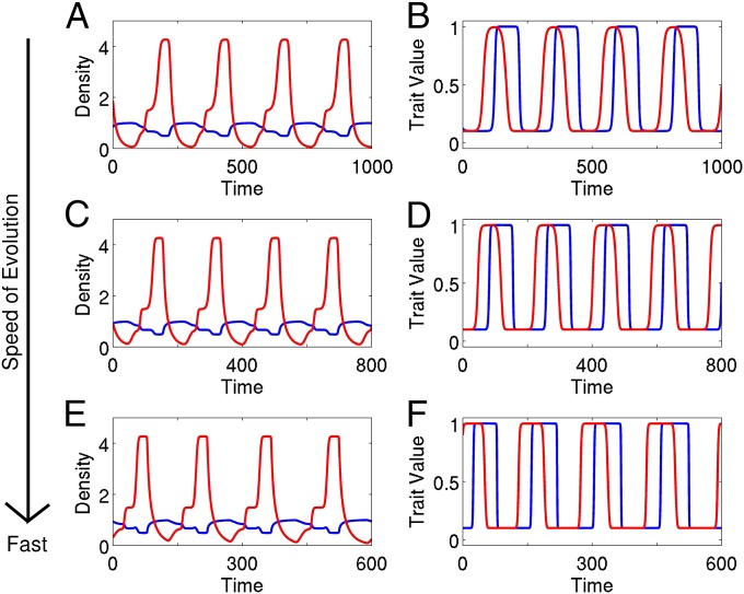
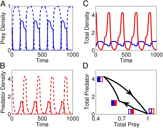
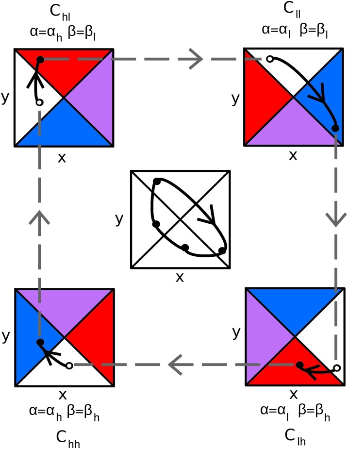
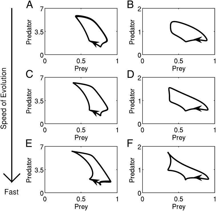
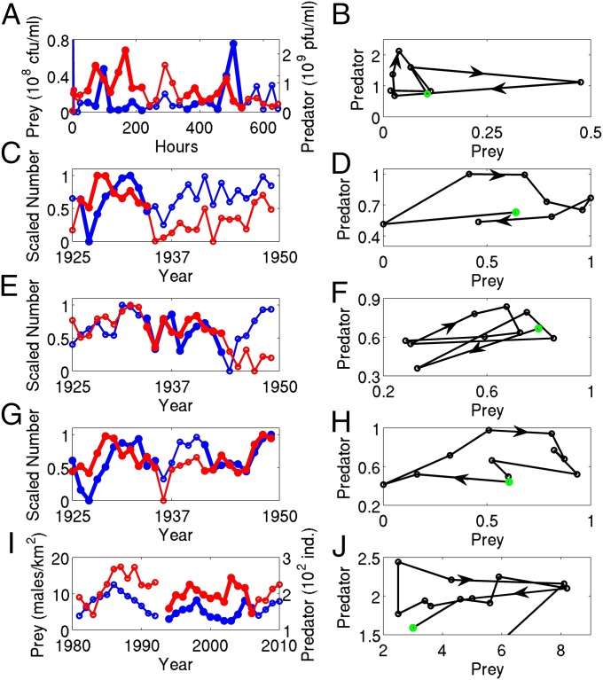
A hallmark of Lotka-Volterra models, and other ecological models of predator-prey interactions, is that in predator-prey cycles, peaks in prey abundance precede peaks in predator abundance. Such models typically assume that species life history traits are fixed over ecologically relevant time scales. However, the coevolution of predator and prey traits has been shown to alter the community dynamics of natural systems, leading to novel dynamics including antiphase and cryptic cycles. Here, using an eco-coevolutionary model, we show that predator-prey coevolution can also drive population cycles where the opposite of canonical Lotka-Volterra oscillations occurs: predator peaks precede prey peaks. These reversed cycles arise when selection favors extreme phenotypes, predator offense is costly, and prey defense is effective against low-offense predators. We present multiple datasets from phage-cholera, mink-muskrat, and gyrfalcon-rock ptarmigan systems that exhibit reversed-peak ordering. Our results suggest that such cycles are a potential signature of predator-prey coevolution and reveal unique ways in which predator-prey coevolution can shape, and possibly reverse, community dynamics.

Keywords: community ecology; eco-coevolutionary dynamics; fast–slow dynamics; population biology.

Fig. 1.

Examples of different kinds of predator–prey cycles. (A) Counterclockwise lynx–hare cycles (3). (B) Antiphase rotifer–algal cycles (8). (C) Cryptic phage-bacteria cycles (9). In all time series, red and blue correspond to predator and prey, respectively. See SI Text, section C for data sources.

Fig. 2.

The qualitative characteristics of the ecological time series from continuous trait model 2 remain the same as the speed of evolution increases. (A, C, and E) Predator (red) and prey (blue) densities. (B, D, and F) Mean predator (offense, red) and mean prey (vulnerability, blue) traits. The speed of evolution is (A and B) as fast, (C and D) two times as fast, and (E and F) five times as fast as the ecological dynamics of the system. In A–F, prey exhibit logistic growth in the absence of predation, predation rates are Type II functional responses, and predators have a linear death rate; see SI Text, section D for equations and parameters.

Fig. 3.

Example of a clonal model exhibiting clockwise predator–prey cycles. (A) Low- (dashed blue) and high- (solid blue) vulnerability prey densities. (B) Low- (dashed red) and high- (solid red) offense predator densities. (C) Total prey (blue) and total predator (red) densities. (D) Total prey and predator densities exhibit clockwise cycles in the phase plane; arrows denote the flow of time. Blue and red rectangles denote the frequencies of the prey and predator clonal types along the cycle, respectively. In the rectangles, open areas correspond to the frequency of low-vulnerability or low-offense clones and filled areas correspond to the frequency of high-vulnerability or high-offense clones. Simulations are of clonal model 1 with logistic growth of the prey clones, Type II functional responses, and linear predator mortality rates; see SI Text, section D for equations and parameters.

Fig. 4.

When evolution is nearly instantaneous, eco-evolutionary cycles can be decomposed into slow ecological dynamics and fast evolutionary jumps. Slow population dynamics (solid black curves) occur on four critical manifolds (x,y planes labeled “$C_{ij}$” in the corners). The critical manifolds are defined by fixing the mean prey (α) and mean predator (β) traits at their low (l) or high (h) values. White regions in the planes are evolutionary attractors and colored regions evolutionary repellers in the α-direction (red), the β-direction (blue), or both directions (purple). Fast evolutionary dynamics (dashed gray lines) occur as solutions jump between the critical manifolds. Solutions behave in the following way. A solution lands in the white region of a critical manifold (open circle) and then moves (solid black curves) toward the attracting equilibrium point on that manifold (filled circle). After crossing into a colored region of the manifold, the solution jumps to the white region of another critical manifold (dashed gray line). Repeating and concatenating the population dynamics on each critical manifold yields the eco-coevolutionary cycle in the center.

Fig. 5.

Two examples of clockwise predator–prey cycles. The speed of evolution is (A and B) as fast, (C and D) two times as fast, and (E and F) five times as fast as the ecological dynamics of the system. Simulations are of continuous trait model 2 where the prey exhibit logistic growth in the absence of predation and predation rates follow a Type II functional response. In A, C, and E, the predators have a linear death rate and in B, D, and F the predators have a nonlinear death rate; see SI Text, section D for equations and parameters.

Fig. 6.

Examples of clockwise predator–prey cycles from (A and B) phage–cholera chemostat experiments (38), (C–H) mink and muskrat trapping data from the Hudson’s Bay Company (40), and (I and J) gyrfalcon and rock ptarmigan census data (39). (A, C, E, G, and I) Predator (red) and prey (blue) time series. (B, D, F, H, and J) Thickened segments of time series plotted in the phase plane. Arrows denote the flow of time and green circles denote the first time point. Only the first thickened segments of A and G are plotted in B and H; see SI Text, section C for the second segments. CFU, colony-forming unit; PFU, plaque-forming unit. See SI Text, section C for data sources.

References

1. Elton CS. Periodic fluctuations in the number of animals: Their causes and effects. J Exp Biol. 1924;2:119–163.
1. Gause GF. Experimental demonstration of Volterra’s periodic oscillations in the numbers of animals. J Exp Biol. 1935;12(1):44–48.
1. Elton CS, Nicholson M. Fluctuations in numbers of the muskrat (Ondatra zibethica) in Canada. J Anim Ecol. 1942;11(1):96–126.
1. Rosenzweig ML, MacArthur RH. Graphical representation and stability conditions of predator-prey interactions. Am Nat. 1963;97(895):209–223.
1. Lotka AJ. 1934. Théorie analytique des associations biologiques, Hermann, Paris.
Publication types