Space-time wiring specificity supports direction selectivity in the retina

Abstract

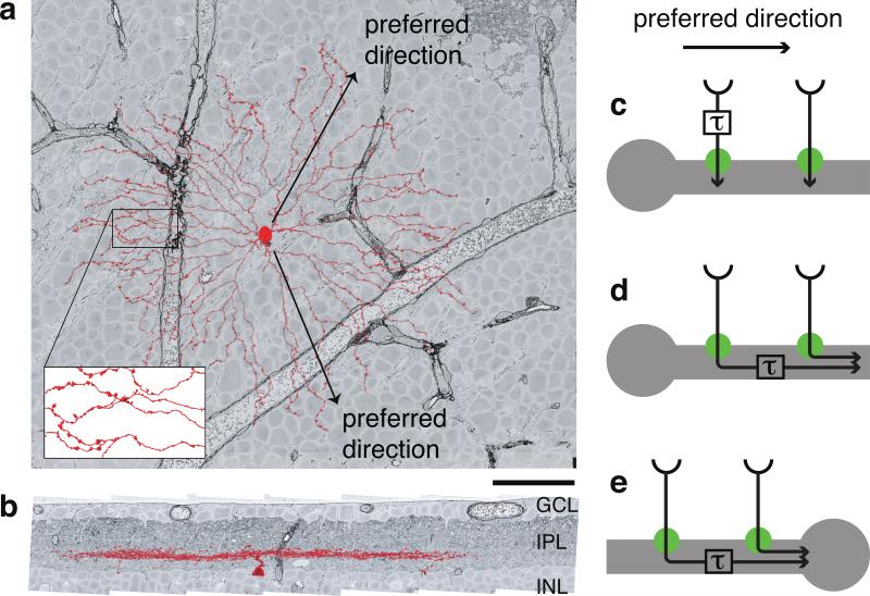
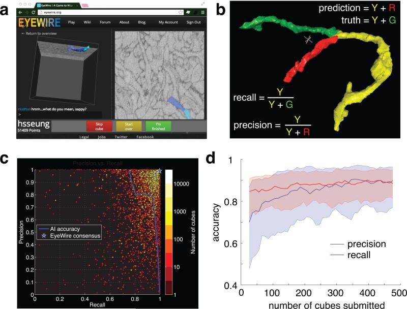
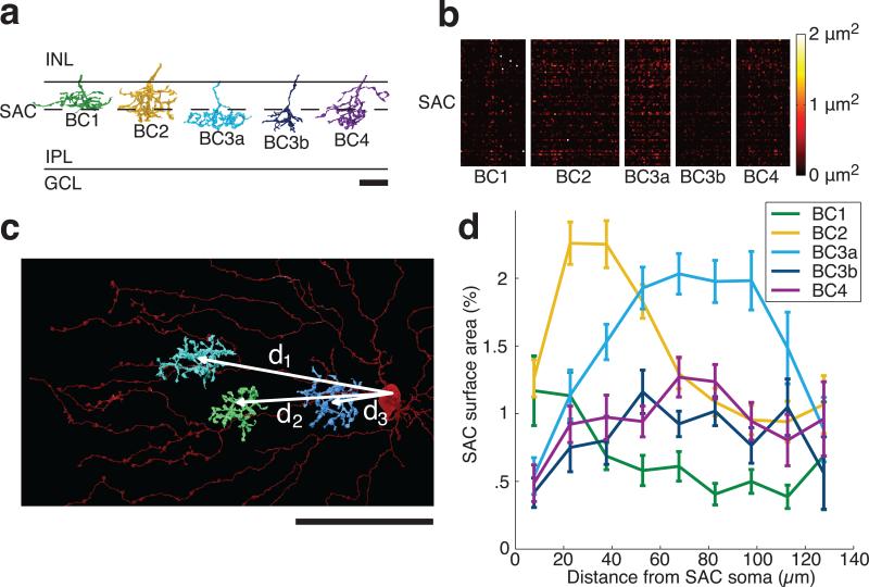
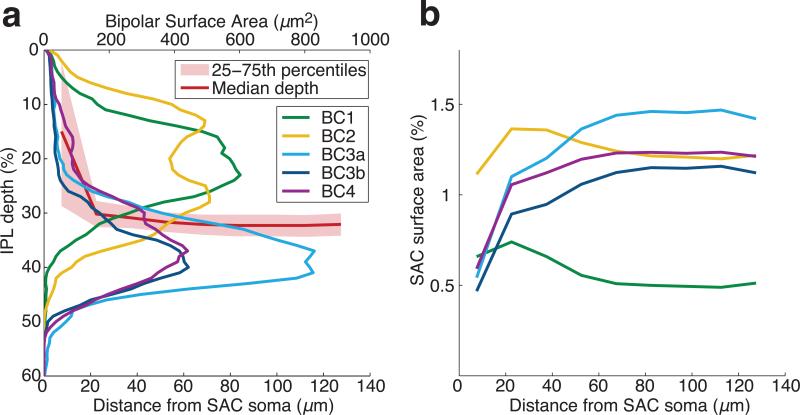
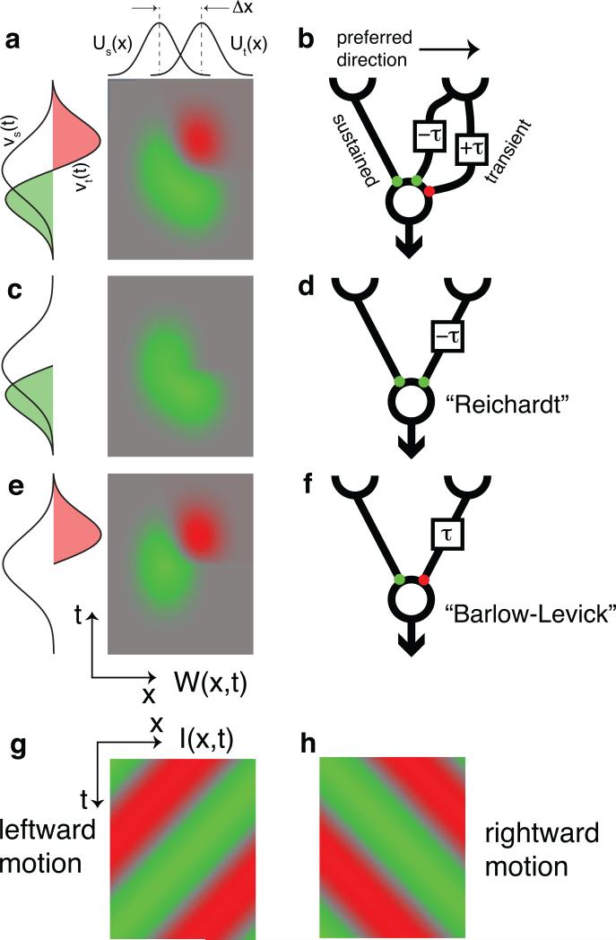
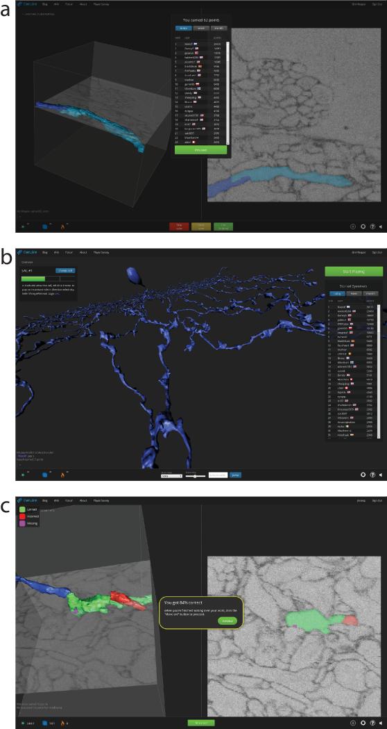
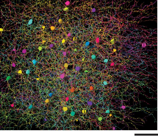
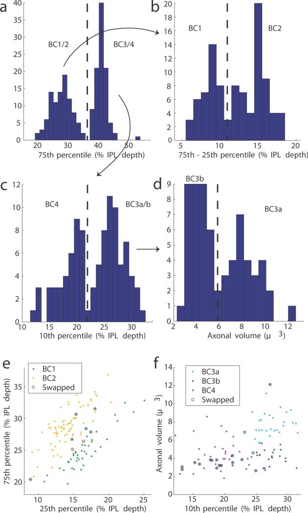
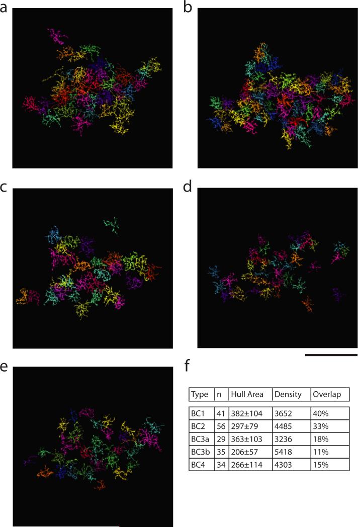
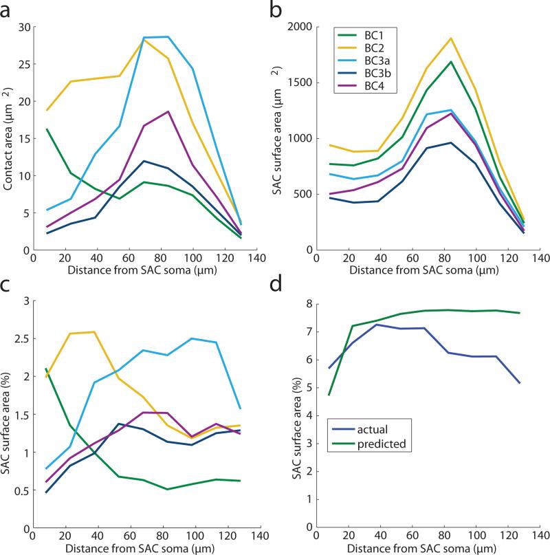
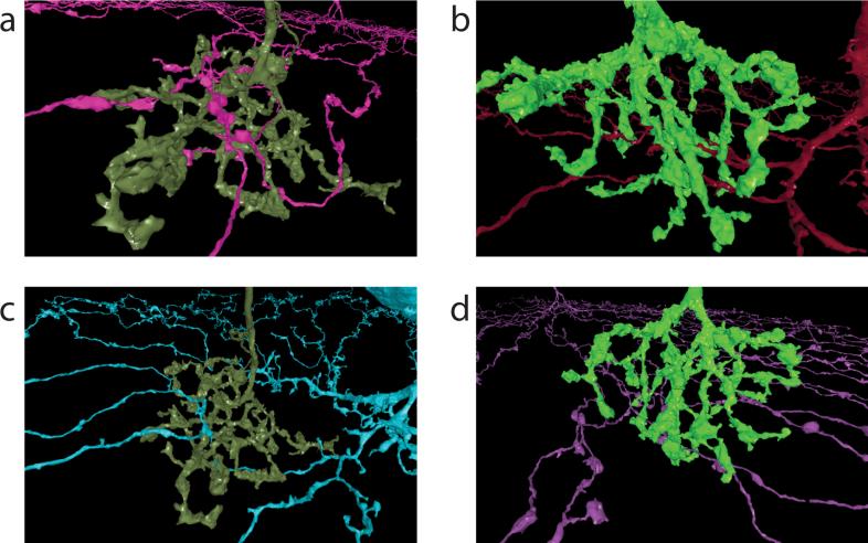
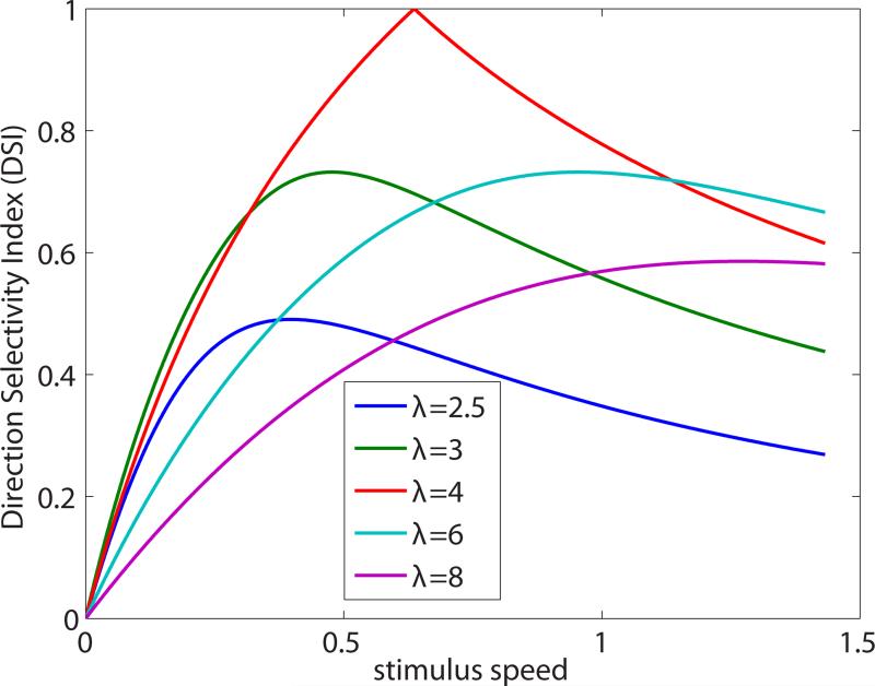
How does the mammalian retina detect motion? This classic problem in visual neuroscience has remained unsolved for 50 years. In search of clues, here we reconstruct Off-type starburst amacrine cells (SACs) and bipolar cells (BCs) in serial electron microscopic images with help from EyeWire, an online community of 'citizen neuroscientists'. On the basis of quantitative analyses of contact area and branch depth in the retina, we find evidence that one BC type prefers to wire with a SAC dendrite near the SAC soma, whereas another BC type prefers to wire far from the soma. The near type is known to lag the far type in time of visual response. A mathematical model shows how such 'space-time wiring specificity' could endow SAC dendrites with receptive fields that are oriented in space-time and therefore respond selectively to stimuli that move in the outward direction from the soma.

Figure 1. Starburst amacrine cell and its direction selectivity

Off SAC (red) viewed opposite (a) and perpendicular (b) to the light axis. GCL, IPL, INL are ganglion cell, inner plexiform, inner nuclear layers. Grayscale images from the e2198 dataset. Swellings of distal dendrites are presynaptic boutons (inset). Scale bar is 50 μm. c, We hypothesize that a SAC dendrite is wired to pathways with different time lags of visual response. d, A previous model invoked the time lag due to signal conduction in a passive dendrite. e, The previous model predicts an inward preferred direction for the somatic voltage, contrary to empirical observations.

Figure 2. EyeWire combines crowd and artificial intelligence

a, 3D and 2D views in the neuron reconstruction game. b, Precision and recall are two measures of accuracy. c, Accuracy of artificial intelligence (AI), 5881 EyeWirers, and EyeWirer consensus on reconstruction of a ganglion cell. d, EyeWirer precision and recall increase with number of cubes submitted. Solid lines are median values across 208 EyeWirers who submitted at least 500 cubes, and shaded regions indicate 25th to 75th percentile.

Figure 3. 3D reconstructions of Off BCs and SACs

Cells viewed opposite the light axis. a, BCs alone. b, BCs with SACs. Scale bar is 50 μm.

Figure 4. BC-SAC contact

a, Off BCs were divided into five types^,, based on IPL depth and size. Scale bar is 10 μm. b, Contact areas of BC-SAC pairs, sorted by BC types. c, Pairs were further sorted by the distance of the BC axon from the SAC soma, as measured in the tangential plane. Scale bar is 50 μm. d, Average BC-SAC contact vs. distance, normalized to percentage of SAC surface area at that distance (Extended Data Fig. 3b). Standard error is based on the number of pairs for each BC type and distance.

Figure 5. BC-SAC co-stratification

a, SAC dendrites move deeper into the IPL (median depth, red line) with increasing distance from the SAC soma in the tangential plane. Stratification profiles of BC types, defined as density of surface area over the depth of the IPL. b, Co-stratification predictions of BC-SAC contact area vs. distance from the SAC soma. The curves are normalized by SAC area at each distance, and are therefore directly comparable with those of Figure 4d.

Figure 6. Mathematical model of the BC-SAC circuit

a, Spatiotemporal filter of Eq. (2). Green is positive, red is negative, and gray is zero. b, The transient pathway effectively combines a positive channel that leads the sustained pathway by τ and a negative channel that lags by τ. c, Removing the negative channel yields a Reichardt detector (d). e, Removing the positive channel yields a Barlow-Levick detector (f). A moving visual stimulus I(x,t) is oriented in space-time (g, h), and so are the spatiotemporal filters (a, c, e).

Extended Data Figure 1. EyeWire screenshots

a, Numerical score after gameplay of a cube, with leaderboard below. b, Overview mode with neuron under reconstruction (center), global chat (bottom left), progress bar for neuron (upper left), leaderboard (right), settings and help (bottom right). c, Tutorial play.

Extended Data Figure 2

Questionnaire administered to EyeWirers.

Extended Data Figure 3. EyeWire demographics

Data based on 729 responses to the questionnaire in Extended Data Fig. 2. Age distribution of (a) all respondents and (b) those among the top 100 players ranked by number of cubes submitted. c, Gender distribution of all respondents and those among the top 100 players. d, Distribution of educational levels.

Extended Data Figure 4. Entirety of reconstructed SACs

Only the central region of this plexus of SAC dendrites is portrayed in Figure 3b. Scale bar is 50 μm.

Extended Data Figure 5. Clustering procedure for BCs

a, Cells were divided by the 75th percentile of their stratification profiles. b, The shallow cluster BC1/2 was separated into BC1 and BC2 using stratification width, defined as the difference between 75th and 25th percentiles. c, The deep cluster BC3/4 was divided by 10th percentile into BC4 and BC3. d, BC3 was divided by axonal volume to yield BC3a and BC3b. Scatter plots of the (e) BC1/2 and (f) BC3/4 divisions show swaps made to eliminate mosaic violations. No swaps between BC1/2 and BC3/4 were needed.

Extended Data Figure 6. Mosaics of Off BC types

Reconstructed BCs of types 1, 2, 3a, 3b, and 4 (a through e, respectively). BC1/2 mosaics appear complete. BC3/4 mosaics show some gaps, probably because some thin axons were missed in the INL (Methods). Scale bar is 50 μm. f, Statistics of BC types. Means and standard deviation of the hull area (area of the convex hull around the cell) are in μm². Type densities are the number of cells (n) divided by the area of the union of hulls of that cell type, and are in cells/mm² without compensation for tissue shrinkage (Methods). Our densities resemble those of Wassle et al. (2009), who found 2233, 3212, 1866, 3254, and 3005 cells/mm².

Extended Data Figure 7. Alternative contact analysis

Analysis based on summing over BC-SAC pairs rather than averaging as in main text. a, Total BC-SAC contact vs. distance from the SAC soma. b, Total SAC area within the union of convex hulls of each BC type versus distance. The peak at 80 μm is the location of maximum dendritic branching. The sharp decrease at larger distances is due to thinning and termination of branches. The graphs differ across BC types, which in our sample do not cover exactly the same retinal areas. c, Fraction of SAC area in contact with BC types, estimated by dividing contact area (a) by SAC area (b). This estimate is similar to that of Figure 4d, but lacks error bars. d, Fraction of SAC area contacted by all BC types, the sum of the contact fractions in (c). Also plotted is the contact predicted by co-stratification, the sum of the curves from Figure 5b.

Extended Data Figure 8. Proximity versus contact

Neurons that intermingle may or may not contact each other. a, b. Type 2 and 3a BCs (respectively) contacting SACs. The cells are roughly 24 and 21 μm wide. c, d. Other SACs are well within the arbors of the same two BCs, yet make no contact at all.

Extended Data Figure 9. Model direction selectivity index (DSI) versus stimulus speed

The graphs are for traveling sine waves of various wavelengths λ (units of Δx). Speed is in units of Δx/τ. The preferred speed (horizontal location of each peak) is λ/(2π). Note that responses are cut off at high speeds by the temporal filters of the model, but the DSI can decay more slowly.

References

1. Borst A, Euler T. Seeing things in motion: models, circuits, and mechanisms. Neuron. 2011;71:974–94. - PubMed
1. Vaney DI, Sivyer B, Taylor WR. Direction selectivity in the retina: symmetry and asymmetry in structure and function. Nat. Rev. Neurosci. 2012;13:194–208. - PubMed
1. Euler T, Detwiler PB, Denk W. Directionally selective calcium signals in dendrites of starburst amacrine cells. Nature. 2002;418:845–52. - PubMed
1. Hausselt SE, Euler T, Detwiler PB, Denk W. A dendrite-autonomous mechanism for direction selectivity in retinal starburst amacrine cells. PLoS Biol. 2007;5:e185. - PMC - PubMed
1. Yonehara K, et al. The first stage of cardinal direction selectivity is localized to the dendrites of retinal ganglion cells. Neuron. 2013;79:1078–85. - PubMed
Publication types