Fast spatiotemporal image reconstruction based on low-rank matrix estimation for dynamic photoacoustic computed tomography

Abstract

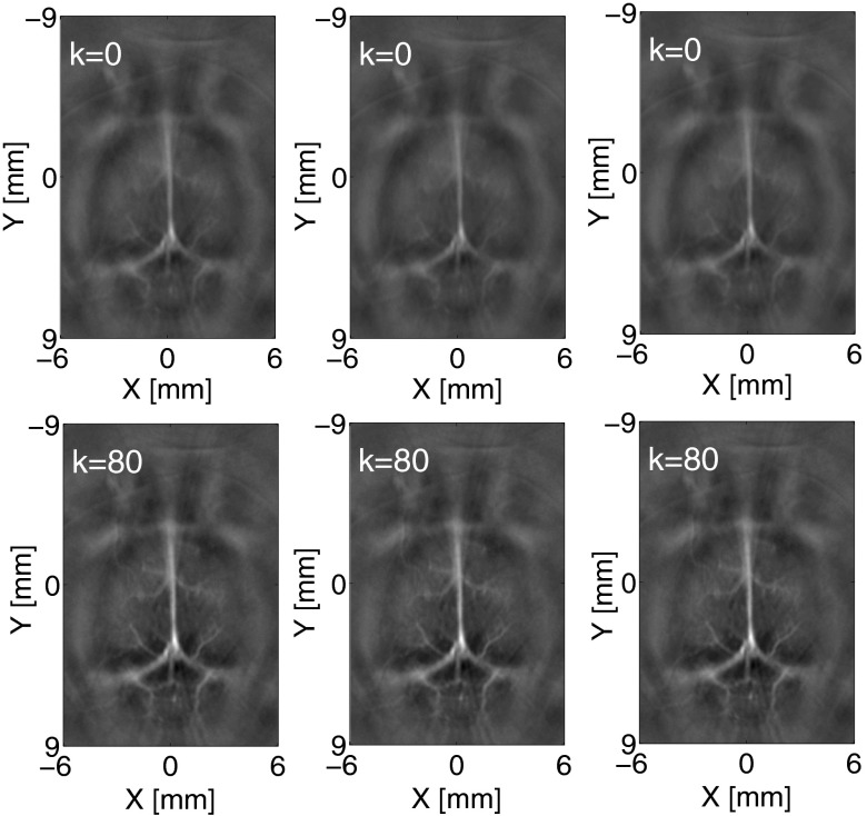
In order to monitor dynamic physiological events in near-real time, a variety of photoacoustic computed tomography (PACT) systems have been developed that can rapidly acquire data. Previously reported studies of dynamic PACT have employed conventional static methods to reconstruct a temporally ordered sequence of images on a frame-by-frame basis. Frame-by-frame image reconstruction (FBFIR) methods fail to exploit correlations between data frames and are known to be statistically and computationally suboptimal. In this study, a low-rank matrix estimation-based spatiotemporal image reconstruction (LRME-STIR) method is investigated for dynamic PACT applications. The LRME-STIR method is based on the observation that, in many PACT applications, the number of frames is much greater than the rank of the ideal noiseless data matrix. Using both computer-simulated and experimentally measured photoacoustic data, the performance of the LRME-STIR method is compared with that of conventional FBFIR method followed by image-domain filtering. The results demonstrate that the LRME-STIR method is not only computationally more efficient but also produces more accurate dynamic PACT images than a conventional FBFIR method followed by image-domain filtering.

Fig. 1

Slow-time frames of the images reconstructed by the use of spatiotemporal image reconstruction (STIR) from simulated noise-free data (Video 1, QuickTime 164 KB) [URL: http://dx.doi.org/10.1117/1.JBO.19.5.056007.1].

Fig. 2

Pixel time activity curves (TACs) of the phantom (solid) and of the images reconstructed by using STIR from noise-free data (circle), where blue, red, green, and black correspond to the pixels marked by A, B, C, and D in Fig. 1, respectively.

Fig. 3

Sixtieth slow-time frames of (a) the phantom, and the images reconstructed by using (b) the frame-by-frame image reconstruction (FBFIR)-Hann, (c) the FBFIR-PCA, and (d) the low-rank matrix estimation-based STIR (LRME-STIR) methods, respectively, from the noisy data contaminated with 20% Gaussian white noise (Video 2, QuickTime 258 KB) [URL: http://dx.doi.org/10.1117/1.JBO.19.5.056007.2]. The gray-scale window is $[-0.1,1.1]$.

Fig. 4

Estimates of ${\{A_k(x,y=0)\}}_{k=0}^{89}$ by using (b) the FBFIR-Hann method, (c) the FBFIR-PCA method, and (d) the LRME-STIR method from the noisy data contaminated with 20% Gaussian white noise, respectively. The original phantom is plotted in panel (a). The gray-scale window is $[-0.1,1.1]$.

Fig. 5

Pixel TACs of the phantom (solid) and of the images reconstructed by using (a) FBFIR-Hann, (b) FBFIR-PCA, and (c) LRME-STIR, respectively, from the noisy data contaminated with 20% Gaussian white noise. Blue, red, green, and black correspond to the pixels marked by A, B, C, and D in Fig. 1, respectively.

Fig. 6

Plots of the mean squared errors (MSE’s) of reconstructed images versus the noise levels.

Fig. 7

The singular value spectra of the measured raw data $\underset{\_}{\mathbf{P}}$.

Fig. 8

Slow-time frames of the images reconstructed from the experimental raw data by using the FBFIR (top row) and the LRME-STIR (bottom row) methods, respectively (Video 3, QuickTime 262 KB) [URL: http://dx.doi.org/10.1117/1.JBO.19.5.056007.3]. The gray-scale window is $[-2.2,5.3]$.

Fig. 9

Estimates of ${\{A_k(x=0,y)\}}_{k=0}^{89}$ reconstructed by using (a) the FBFIR method and (b) the LRME-STIR method from the experimental raw data, respectively. The gray-scale window is $[-2.2,5.3]$.

Fig. 10

Pixel TACs of the images reconstructed from experimental raw data by using the FBFIR (solid) and the LRME‐STIR (circles) methods, respectively. Blue, red, green, and black correspond to the pixels marked by A, B, C, and D in Fig. 8, respectively.

Fig. 11

Slow-time frames of the images reconstructed from the high-noise data set (Video 4, QuickTime 262 KB) [URL: http://dx.doi.org/10.1117/1.JBO.19.5.056007.4]. Columns from left to right correspond to the FBFIR‐Hann, the FBFIR‐PCA, and the LRME-STIR methods, respectively. The gray-scale window is $[-2.2,5.3]$.

Fig. 12

Estimates of ${\{A_k(x=0,y)\}}_{k=0}^{89}$ reconstructed by using (a) the FBFIR method, (b) the FBFIR-Hann, (c) the FBFIR-PCA, and (d) the LRME-STIR methods from the experimental high-noise data set, respectively. The gray-scale window is $[-2.2,5.3]$.

Fig. 13

Pixel TACs of the reference images (solid) and the images reconstructed by using (a) the FBFIR-Hann, (b) the FBFIR-PCA, and (c) the LRME-STIR methods, respectively, from the experimental data contaminated with computer-simulated noise. Blue, red, green, and black correspond to the pixels marked by A, B, C, and D in Fig. 8, respectively.

References

-
- Wang L. V., “Tutorial on photoacoustic microscopy and computed tomography,” IEEE J. Sel. Topics Quantum Electron. 14, 171–179 (2008).IJSQEN10.1109/JSTQE.2007.913398 - DOI
- Oraevsky A. A., Karabutov A. A., “Optoacoustic tomography,” Chapter 34 in Biomedical Photonics Handbook, Vo-Dinh T., Ed., pp. 34/1–34/34, CRC Press LLC, Boca Raton, FL: (2003).
Publication types
MeSH terms
Grants and funding
LinkOut - more resources
Full Text Sources
Other Literature Sources
Medical
Molecular Biology Databases
Miscellaneous