Understanding brain networks and brain organization

Abstract

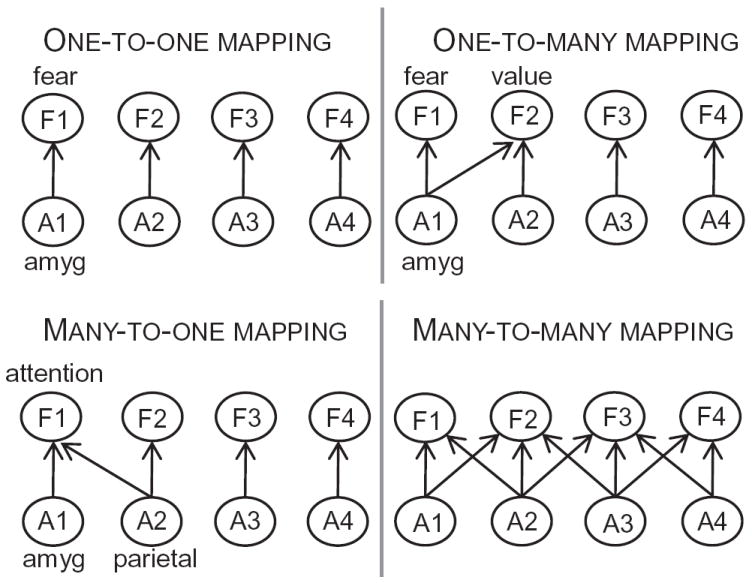
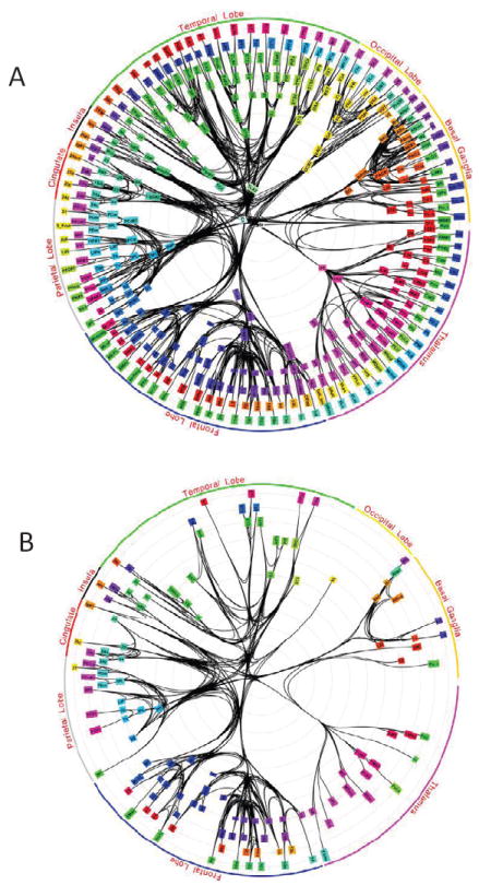
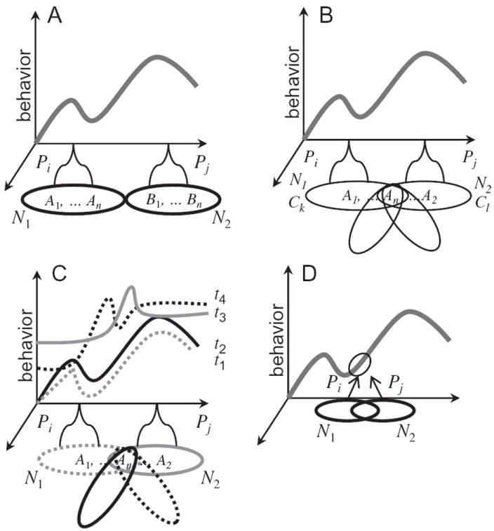
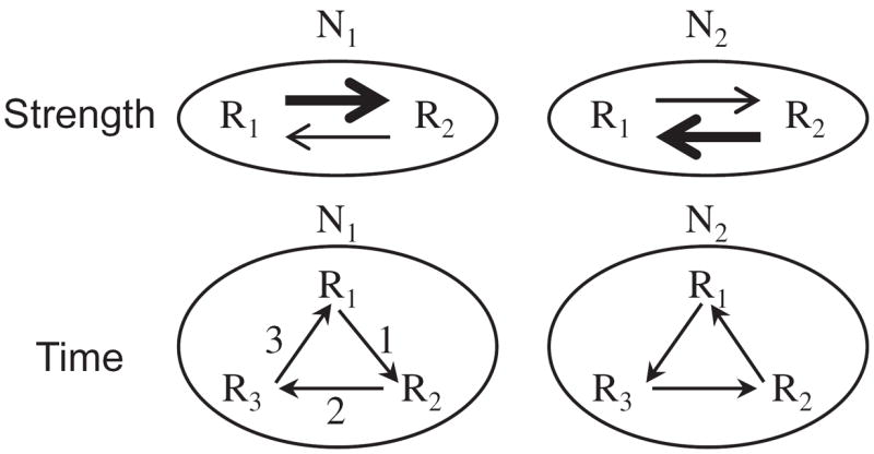
What is the relationship between brain and behavior? The answer to this question necessitates characterizing the mapping between structure and function. The aim of this paper is to discuss broad issues surrounding the link between structure and function in the brain that will motivate a network perspective to understanding this question. However, as others in the past, I argue that a network perspective should supplant the common strategy of understanding the brain in terms of individual regions. Whereas this perspective is needed for a fuller characterization of the mind-brain, it should not be viewed as panacea. For one, the challenges posed by the many-to-many mapping between regions and functions is not dissolved by the network perspective. Although the problem is ameliorated, one should not anticipate a one-to-one mapping when the network approach is adopted. Furthermore, decomposition of the brain network in terms of meaningful clusters of regions, such as the ones generated by community-finding algorithms, does not by itself reveal "true" subnetworks. Given the hierarchical and multi-relational relationship between regions, multiple decompositions will offer different "slices" of a broader landscape of networks within the brain. Finally, I described how the function of brain regions can be characterized in a multidimensional manner via the idea of diversity profiles. The concept can also be used to describe the way different brain regions participate in networks.

Keywords: Brain; Function; Networks; Structure.

Figure 1

Structure-function mapping in the brain. A central argument of the paper is that because the mapping from structure to function is many-to-many, understanding the instantiation of functions by the brain necessitates sophisticated frameworks whose basic elements are networks, not regions. Abbreviations: A1, …, A4: areas 1 to 4; amyg: amygdala; F1, …, F4: functions 1 to 4; Reproduced with permission [2].

Figure 2

Whole-brain network connectivity structure. (A) The analysis considered existing anatomical connectivity data of an extensive set of cortical and subcortical areas spanning most major brain sectors. The basal ganglia refer to nuclei at the base of the forebrain, including the amygdala. (B) Innermost “core” circuit. Notably, several amygdala nuclei were included in the inner core. Reproduced with permission [34].

Figure 3

Structure-function mapping and networks. (A) The “landscape of behavior” displays a caricature of the multidimensional space of behaviors. Abbreviations: A₁, A₂, A_N, B₁, and B_N: brain regions; N₁ and N₂; networks; P_i and P_j: processes. (B) Intersecting networks. The networks C_K and C_L (and the additional ones) intersect at node A_n. (C) Dynamic aspects. Region A_N will have network affiliations that vary as a function of time. Therefore, the processes carried out by the emerging networks will evolve across time and lead to dynamic “landscapes of behavior”. The four time points represented are such t₁ ≅ t₂ but far from t₃ ≅ t₄. (D) Structure-function mappings in the case of networks. Two networks may instantiate similar processes, a case of many-to-one mapping. The reverse relationship is also suggested to apply to networks, namely, one-to-many mappings (see text). Reproduced with permission [2].

Figure 4

Network interactions. The same regions R_i may comprise distinct networks depending on how the regions interact both in terms of strength-across-time (top row) and time (bottom row). For instance, when the R₁ → R₂ link is strong, network N₁ will behave differently from when the R₂ → R₁ link is strong (in that case, the network is being labeled N₂). This could occur, for instance, due to plasticity. The bottom row illustrates that inter-region interactions may follow a different temporal order, thereby leading to different function (in this case, the networks were labeled N₁ and N₂). In both cases, the same network label N₁ could have been used for the two scenarios, with the understanding that N₁ varies as a function of time. Reproduced with permission [2].

Figure 5

Network structure and hub nodes. Nodes with unusually high connectivity may be considered “hubs”, and are likely to have important roles in determining information flow. Reproduced with permission [2].

Figure 6

Network associated with Brodmann’s area 46 in dorsal-lateral PFC. Given its high connectivity, the area can be considered a hub. Reproduced with permission [65].

Figure 7

Conventional and alternative views of thalamo-cortical circuits. In the conventional view, cortical communication is accomplished via pathways between cortical sites. In the alternative view, as proposed by Sherman and colleagues, higher-order thalamic nuclei play a prominent role in this communication, and direct cortico-cortical pathways may be less important. FO, first order; HO, higher order. Reproduced with permission [74].

Figure 8

Prefrontal cortex connectivity. Fraction of frontal areas that receive signals from each modality as a function of the number of connectivity “steps” within frontal cortex. Zero indicates the areas that receive a direct projection from the indicated sensory or motor modality, and one indicates the fraction of areas that would receive the signal after a single step within frontal cortex. Amy, amygdala; Aud, auditory; G/O, gustatory/olfactory; Hip, hippocampus; Mot, motor; MS, multisensory; SS, somatosensory; Vis, visual. Reproduced with permission [38].

Figure 9

Hypothalamic ascending connectivity. Summary of the four major pathways from the hypothalamus to cerebral cortex schematized on a flattened representation of the rat brain. The basal ganglia here refer to the basal forebrain and the amygdala complex. Note that one of the indirect connections first descends to the brainstem. BG, basal ganglia; BS, brainstem; CTX, cortex; HY, hypothalamus; TH, thalamus. Reproduced with permission [29].

Figure 10

Basic plan of the vertebrate brain. From Striedter (2005) with permission. Figure 3.8 The Vertebrate Brain Archetype Schematic drawings of the vertebrate brain region archetype from dorsal (top) and lateral (bottom) perspectives. Some elements have been omitted for the sake of clarity. Abbreviations: C = caudal; Cb = cerebelum; D = dorsal; Dienc. = diencephalon; DT = dorsal thalamus; ET = epitalamus; Hypo. = hypothalamus; nV = trigeminal nerve; nVII = facial nerve; nVIII = octaval nerve; nIX =glossopharyngeal nerve; nX = vagal nerve; P = pretectum; Pit, = posterior pituitary; POA = preoptic area; P. Tub, = posterior tuberculum; R = rostral; Tegm. = tegmentum; V = ventral; VT = ventral thalamus.

Figure 11

Basic plan of the vertebrate brain represented as a “flat” map. Reproduced from Swanson (2007) with permission.

Figure 12

Summary representation of the amygdala in rats (A), monkeys (B), and humans (C). Glial cells, circles; neurons, triangles: rats < monkeys < humans. Neuron density: rats > monkeys > humans. Glia density: rats ¼ monkeys ¼ humans. Glia/neuron ratio: rats < monkeys < humans. Connectivity with visceral and autonomic systems (mainly via the central nucleus): rats ¼ monkeys ¼ humans. Connectivity with cortical systems (between the neocortex and the lateral, basal, and accessory basal nuclei): rats < monkeys < humans. The proportions of the different parameters are not precisely scaled. Reproduced with permission [88].

Figure 13

Function and structure. The relationship between structure and function can be nuanced and complex. While panel (A) describes the “default” case of a structural connection leading to a functional relationship, the other panels describe how the link can be far from straightforward. See text for further discussion. Abbreviations: Ri: regions; Ci: contexts. Reproduced with permission [2].

Figure 14

Emotion alters the response pattern across early visual cortex. (A) Both fearful and neutral (not shown) faces were presented with a ring that indicated whether it was a safe or threat (possible mild shock) condition. (B) Functional connectivity between visual regions V1, V2, V3, and V4 during affective (left) and neutral (right) context as indexed via pairwise correlations (average correlation shown). (C) Correlation matrix of differential responses for fearful vs. neutral faces in both affective and neutral contexts (ring colors). The upper-left part is the same as in panel B. Of the entire matrix, that was the only part that was robustly altered as a function of context. Abbreviations: Varea: correlations within early visual areas; Oarea: correlations within “other areas”; VOarea: correlations between early visual and “other areas”. L: left; R: right; PrCu: precuneus; STS: superior temporal sulcus; IPS: intraparietal sulcus; pSMA: pre-supplementarymotor area; PrCs: precentral sulcus; FEF: frontal eye field; INS: insula. Colors code for correlation values as indicated by the color scale. Adapted with permission [105].

Figure 15

The effects of common efferents, two-step relay, and common afferents on functional connectivity. *P< 0.05, Tukey test. Reproduced with permission [114].

Figure 16

Network structure and reward. (A) Community detection was applied to the set of brain regions that responded more strongly to reward vs. no-reward at the cue phase (see Figure 6.4). Two communities were detected; please see [123] for region abbreviations. (B) Comparison of the pattern of connectivity between reward and no-reward contexts revealed increases during the former. The increases were observed mostly between the two communities, reflecting increased integration with reward. The polar plot shows increases in functional connectivity of the right caudate with nearly all regions belonging to the “other” community. Line width represents the relative strength of the functional connectivity between regions. Adapted with permission [123].

Figure 17

Network structure and threat. (A) Community detection was applied to the set of brain regions that responded more strongly to threat vs. safe at the cue phase (see Figure 5.7). Two communities were detected; please see [123] for region abbreviations. (B) Changes in threat versus safe connectivity for all pairs of regions within the community on the left in panel A. Dark colors indicate no change; warm colors indicate threat greater than safe; cool colors indicate threat smaller than safe. One of the effects of threat may have been to “disconnect” cortical regions from each other, possibly leading to performance impairments. Adapted with permission [123].

Figure 18

Functional fingerprints of regions and networks. (A) The polar plots illustrate the fingerprints of three brain regions. Each vertex corresponds to one of the domains investigated. Both the left anterior insula and the left intraparietal sulcus exhibited diverse functional profiles. The superior temporal gyrus in the vicinity of auditory cortex was less diverse, though the fingerprint revealed its involvement in emotional processing, in addition to audition. (B) The polar plots illustrate the fingerprints of two brain networks, which were defined by Toro et al. [118] based on a meta-analysis of task activation data. The frontal-parietal “attention” network was a task-positive network generated by “seeding” the left intraparietal sulcus. The cingulate-parietal “resting-state” network was a task-negative network generated by “seeding” the ventral-anterior medial PFC. Although both networks are quite diverse, the analysis revealed that they are fairly complementary to one another. Reproduced with permission [153].

Figure 19

Diversity map. (A) Areas of higher diversity are shown in warm colors and areas of lower diversity are shown in cool colors (color bar represents H values). Locations without colors did not have enough studies for the estimation of diversity. Reproduced with permission [153].

Figure 20

Network functional fingerprints. Reproduced with permission [153].

Figure 21

Network comparison. A multivariate comparison with permutation testing was used to compare pairs of networks. The distributions portray the null distribution of possible differences between each pair. The blue vertical bars indicate the observed difference, which is shown on top of each box in terms of its percentile relative to the null distribution (when not shown, the bar was located to the right of the displayed area). For illustration, comparisons with percentiles>95% are shown in red and comparisons with percentiles> 90% are shown in magenta. For example: FrontoParietalN and CinguloParietalN were very different, DorsalAttentionC and VentralAttentionC were distinct but to a lesser extent, and CinguloParietalN and DefaultC were similar. See Table 1 for network explanations. Reproduced with permission [153].

Figure 22

Network assortativity. Assortativity measures the extent to which functional fingerprints from regions of the same network are more similar to each other than to fingerprints from other networks. The percentile scores provide an indication of the degree of assortativity (or dis-assortativity in the case of CinguloParietalN). See Table 1 for network explanations. Reproduced with permission [153].

Figure 23

Overlap between connection partners of each insular subdivision. To facilitate displaying overlap, the corresponding right and left insular subregions were pooled together resulting in three insular subregions (dorsal anterior, ventral anterior, posterior insula). Voxels shown in green-to-red colors were coactive with two of the three subregions (the color bar indicates the strength of overlap, specifically, the smallest value of the two strongest partial correlations). Voxels in blue were coactive across all three subdivisions. Adapted with permission [169].

Figure 24

(A) Coactivation of insula subdivisions. Using data from the Neurosynth database, task-based coactivation profiles were determined for each insular subdivision by moving a searchlight in a voxel-wise manner. The color bar indicates the partial correlation value with the specific insular subregion “seed” when all other subdivisions were also considered. (B) “Common” functional fingerprint of insular subdivisions. The common fingerprint was determined by combining all six insular subregion (see text). All task domains were engaged by each subregion at least some of the time. TOM = theory of mind; MemWork = working memory; MemOther = long-term memory. Adapted with permission [169].

References

1. Shallice T. From neuropsychology to mental structure. New York: Cambridge University Press; 1988.
1. Pessoa L. The Cognitive-Emotional Brain: From Interactions to Integration. Cambridge: MIT Press; 2013.
1. Edelman GM, Gally JA. Degeneracy and complexity in biological systems. Proceedings of the National Academy of Sciences of the United States of America. 2001;98:13763–8. - PMC - PubMed
1. Pessoa L. On the relationship between emotion and cognition. Nature Reviews Neuroscience. 2008;9:148–58. - PubMed
1. Cisek P, Kalaska JF. Neural mechanisms for interacting with a world full of action choices. Annual review of neuroscience. 2010;33:269–98. - PubMed
LinkOut - more resources