Coincidence detection in the medial superior olive: mechanistic implications of an analysis of input spiking patterns

Abstract

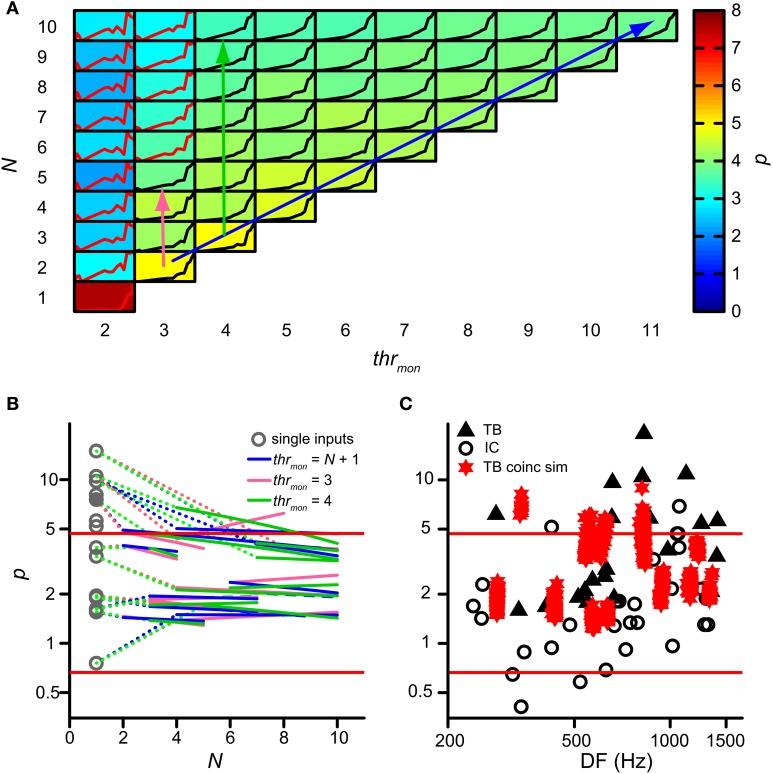
Coincidence detection by binaural neurons in the medial superior olive underlies sensitivity to interaural time difference (ITD) and interaural correlation (ρ). It is unclear whether this process is akin to a counting of individual coinciding spikes, or rather to a correlation of membrane potential waveforms resulting from converging inputs from each side. We analyzed spike trains of axons of the cat trapezoid body (TB) and auditory nerve (AN) in a binaural coincidence scheme. ITD was studied by delaying "ipsi-" vs. "contralateral" inputs; ρ was studied by using responses to different noises. We varied the number of inputs; the monaural and binaural threshold and the coincidence window duration. We examined physiological plausibility of output "spike trains" by comparing their rate and tuning to ITD and ρ to those of binaural cells. We found that multiple inputs are required to obtain a plausible output spike rate. In contrast to previous suggestions, monaural threshold almost invariably needed to exceed binaural threshold. Elevation of the binaural threshold to values larger than 2 spikes caused a drastic decrease in rate for a short coincidence window. Longer coincidence windows allowed a lower number of inputs and higher binaural thresholds, but decreased the depth of modulation. Compared to AN fibers, TB fibers allowed higher output spike rates for a low number of inputs, but also generated more monaural coincidences. We conclude that, within the parameter space explored, the temporal patterns of monaural fibers require convergence of multiple inputs to achieve physiological binaural spike rates; that monaural coincidences have to be suppressed relative to binaural ones; and that the neuron has to be sensitive to single binaural coincidences of spikes, for a number of excitatory inputs per side of 10 or less. These findings suggest that the fundamental operation in the mammalian binaural circuit is coincidence counting of single binaural input spikes.

Keywords: auditory nerve; coincidence detection; coincidence window; input convergence; interaural correlation; interaural time difference; medial superior olive; temporal coding.

Figure 1

Simulation of coincidence detection. (A) Depiction of one run of the coincidence process. In this example, N = 4, thr_mon = 3, thr_bin = 2 and cw = 50 μs. See text for details. (B) Example of pseudobinaural NDF. The traces shown are the average rates of 3 real runs with the same parameters as in (A). Colors correspond to those of the spike trains in (A). Data from a TB fiber with a CF of 559 Hz (SR 1.27 spikes/s). (C) Example of rICF, obtained by choosing responses to noise tokens with different intertoken correlations as inputs on the “ipsilateral” and “contralateral” side. Same fiber and parameters as in (B).

Figure 2

Fitting procedure of NDFs to estimate DF and BW. Dashed lines indicate filter model. Blue lines represent ρ = 1, black lines represent ρ = −1. See text for detailed explanation of steps (A–H).

Figure 3

Data from binaural cells used to constrain simulation output. Red dashed lines indicate the parameter range accepted for coincidence simulation output (see text for details). (A) Scatter plot of bandwidth vs. DF for cat IC datasets (circles; n = 68). (B) Power of rICF as a function of DF for cat IC (n = 29). Data in (A) and (B) taken from (Mc Laughlin et al., 2008, 2014). (C) Histogram of peak firing rate of chinchilla LL noise delay functions (n = 30). (D) Histogram of modulation depth of the same chinchilla LL datasets (n = 30). (E) Scatter plot of halfwidth of central peak of noise delay function as a function of CF or DF, for chinchilla LL fibers (n = 28). (F) ISI histogram for chinchilla LL fibers (n = 35). Only units where the proportion of spikes with ISI < 0.5 ms is smaller than 0.01% of the total number of spikes are included. Vertical dashed line indicates the chosen refractory period in the coincidence counting scheme. Data in (C–F) from Bremen and Joris (2013).

Figure 4

Simulation output for TB dataset. CF = 559 Hz. thr_bin = 2 and cw = 50 μs. (A) NDFs to correlated noise, for several values of N and thr_mon. For each subplot, delay (abscissa) ranges from −2.94 to 2.94 ms, and coincidence rate (ordinate) ranges from 0 to 170 spikes/s. Black traces indicate accepted simulations, red traces indicate unaccepted simulations (i.e., simulations that fail on at least one acceptance criterion, either for NDF or rICF). (B) rICFs for the same dataset and simulation parameters as in (A). For each subplot, the abscissa ranges from ρ = −1 to 1, and the ordinate ranges from 0 to the maximal spike rate of each rICF.

Figure 5

Simulation output for AN dataset. CF = 544 Hz. thr_bin = 2 and cw = 50 μs. (A) NDFs to correlated noise of simulations for one AN dataset, for several N and thr_mon. For each subplot, delay (abscissa) ranges from −2.94 to 2.94 ms, and coincidence rate (ordinate) ranges from 0 to 125 spikes/s. (B) rICFs for the same dataset and simulation parameters as in (A). For each subplot, the abscissa ranges from ρ = −1 to 1, and the ordinate ranges from 0 to the maximal spike rate of each rICF.

Figure 6

Acceptance criteria responsible for failure of simulations (A,B). Acceptance criteria responsible for failure of simulations with one unilateral input less than the minimally required N. Only criteria involved in at least one simulation failure are shown. The proportion of failed simulations due to each criterion is shown for all datasets. Each box is bordered by the upper and lower quartile, and the median is indicated by a red line. The whiskers indicate a range of 1.5 times the interquartile range. The plusses indicate values lying beyond this range. (A) TB fibers (n = 10). (B) AN fibers (n = 12). ul, upper limit; ll, lower limit. (C,D) Criteria responsible for acceptance failure of simulations with thr_mon one lower than the minimally required value. (C) TB fibers (n = 12). (D) AN fibers (n = 12). (E,F) Criteria responsible for acceptance failure of simulations with thr_bin one higher than the maximally accepted value. (E) TB fibers (n = 12). (F) AN fibers (n = 12).

Figure 7

Effect of convergence of inputs on p of rICF. (A) Set of simulations for one TB dataset (same as in Figure 4). N and thr_mon are varied; thr_bin = 2 and cw = 50 μs. In each subplot the rICF corresponding to that combination of simulation parameters is shown. Black traces represent accepted simulation results. Subplot background color represents the power value. The abscissa in each plot ranges from −1 to 1; the ordinate ranges from 0 to the maximum of the particular rICF. (B) TB population data showing change of power with convergence of inputs. Gray circles represent the power for the simulations corresponding to the single input correlograms. Colored lines are fit through accepted simulations, where different colors correspond to the arrows in (A). Dotted lines connect the power of the single input correlogram to these fits. (C) Comparison of power p of rICFs: IC data (circles) are repeated from Figure 3B. TB data (triangles) taken from (Mc Laughlin et al., 2014). Values of p for otherwise accepted simulations (red stars) are added for 13 TB datasets. Solid red lines represent limits of accepted power values (Figure 3B).

Figure 8

Compression of rICF with convergence of inputs. (A,B) The same TB dataset as in Figure 4 is shown. In all cases, thr_bin = 2 and cw = 50 μ s. rICFs are for simulations with N = 3 (circles) and N = 8 (crosses). (A) Simulations for output without monaural coincidences. thr_mon is 4 and 9, respectively. The power p of the fit is stated in the caption. (B) rICFs with the same number of inputs as in (A), but now the thr_mon is fixed at 4. The ordinate in (B) is the same as in (A). Dashed lines show the fits. (C) The average number of input events per successful output spike, as a function of ρ. Five TB datasets were selected that show the largest decrease in p with N, for thr_mon = 3 or 4. Crosses correspond to the high N (lowest p), circles correspond to the low N (highest p). CF is indicated in each panel.

Figure 9

Minimal values of thr_mon of accepted simulation cases. Simulations with TB (A) (n = 12) and AN (B) (n = 13) datasets. Different colors represent different values of thr_bin. Each symbol represents the minimal thr_mon values for the accepted cases of one dataset. Black circles filled with red represent dataset in Figure 4. Symbols are jittered to decrease overlap. cw = 50 μs.

Figure 10

Graphical display of the argument of Colburn et al. (1990). See text for detailed explanation. (A) Number of combinations for either 4 (circles) or 2 (crosses) coincidences, as a function of N. Green traces indicate the possible number combinations monaurally, i.e., twice the number of combinations of either x = 2 or 4 out of N. Black traces indicate the total (monaural + binaural) possible number of combinations, i.e., either 2 or 4 out of 2N. (B) Probability of having exactly 4 coincidences monaurally (green trace), binaurally (blue trace) or in total (black trace), as a function of N. The chance of having an event on 1 input is p_s = 0.0075. (C) Probability of having exactly 2 coincidences monaurally (green trace), binaurally (blue trace) or in total (black trace), as a function of N.

Figure 11

TB simulation output for several N and thr_bin. CF 456 Hz; SR 89.9 Hz; thr_mon = 4; cw = 50 μs. (A) NDFs. The abscissa in each subplot ranges from −2.94 to 2.94 ms. The ordinate in each subplot ranges from 0 to 150 Hz. (B) rICFs. The abscissa in each subplot ranges from −1 to 1. The ordinate in each subplot ranges from 0 to 150 Hz. N and thr_bin are the same in (A) and (B).

Figure 12

Maximal values for thr_bin, for different values of N and thr_mon. (A) TB fibers (n = 12), cw = 50 μs. Black triangles filled with green indicate dataset in Figure 11. (B) AN fibers (n = 13), cw = 50 μs. (C) TB fibers (n = 13), cw = 150 μs. (D) TB fibers (n = 13), cw = 250 μs. Symbols are jittered to decrease overlap.

Figure 13

Simulated NDFs for TB datasets, for different values of cw. In every panel NDFs are shown for one TB dataset, for cw = 50 μs (blue), cw = 150 μs (green) and cw = 250 μs (red). CF and SR are indicated for each dataset. Range of abscissa and ordinate indicated in lower left panel apply to all panels. thr_bin = 2. N and thr_mon for each TB dataset are the minimal values to get an acceptable simulation for cw = 50 μs. Asterisks indicate simulations where the NDFs for cw = 150 μs and cw = 250 μs were not accepted.

Figure 14

Average spike rate at NDF peak for TB (A) and AN (B) simulations. The color of each subplot indicates the average peak rate for accepted simulations with thr_mon and N indicated respectively by the abscissa and ordinate. cw = 50 μs, and thr_bin = 2. Color scale is the same in (A) and (B). The number in each subplot indicates which proportion (in %) of the individual datasets had at least one accepted simulation for that combination of parameters.

Figure 15

Average NDF modulation depth for TB (A) and AN (B) simulations. The color of each subplot indicates the average peak rate for accepted simulations with thr_mon value and N indicated by the abscissa and ordinate. cw = 50 μs, and thr_bin = 2. Color scale is the same in (A) and (B). The number in each subplot indicates which proportion (in %) of the individual datasets had at least one accepted simulation for that combination of parameters.

References

1. Agmon-Snir H., Carr C. E., Rinzel J. (1998). The role of dendrites in auditory coincidence detection. Nature 393, 268–272 10.1038/30505 - DOI - PubMed
1. Albeck Y., Konishi M. (1995). Reponses of neurons in the auditory pathway of the barn owl to partially correlated binaural signals. J. Neurophysiol. 74, 1689–1700 - PubMed
1. Ashida G., Funabiki K., Carr C. E. (2013). Biophysical basis of the sound analogue membrane potential that underlies coincidence detection in the barn owl. Front. Comput. Neurosci. 7:102 10.3389/fncom.2013.00102 - DOI - PMC - PubMed
1. Ashida G., Funabiki K., Kuokkanen P. T., Kempter R., Carr C. E. (2012). Signal-to-noise ratio in the membrane potential of the owl's auditory coincidence detectors. J. Neurophysiol. 108, 2837–2845 10.1152/jn.00366.2012 - DOI - PMC - PubMed
1. Baumann V. J., Lehnert S., Leibold C., Koch U. (2013). Tonotopic organization of the hyperpolarization-activated current (Ih) in the mammalian medial superior olive. Front. Neural Circuits 7:117 10.3389/fncir.2013.00117 - DOI - PMC - PubMed
Publication types
LinkOut - more resources