. 2014 May 13;9(5):e96856.
doi: 10.1371/journal.pone.0096856. eCollection 2014.

Quantification of blood flow and topology in developing vascular networks

Affiliations

Quantification of blood flow and topology in developing vascular networks

Astrid Kloosterman et al. PLoS One. .

Abstract

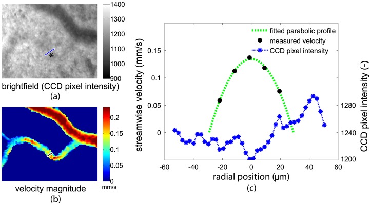
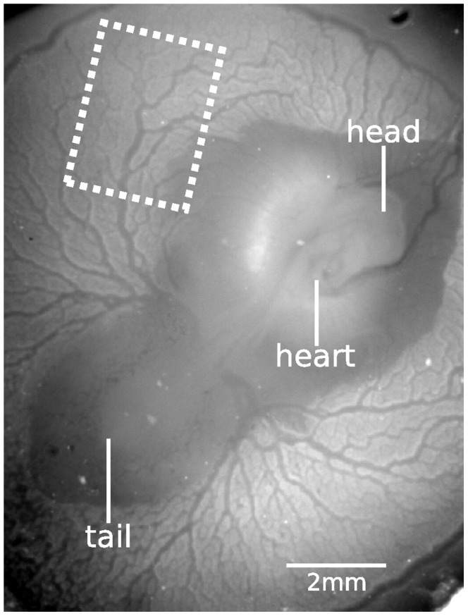
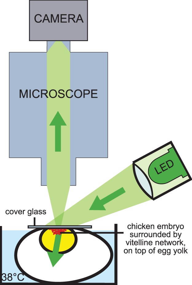
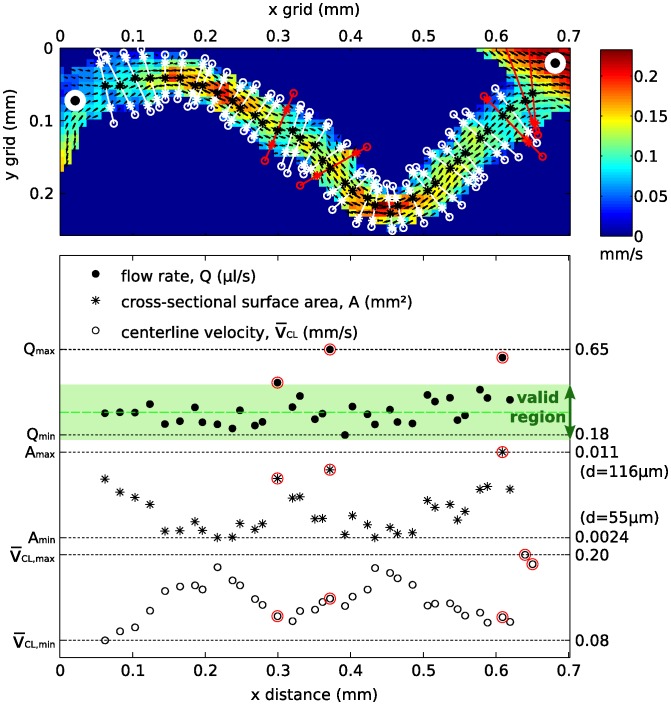
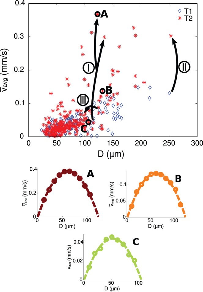
Since fluid dynamics plays a critical role in vascular remodeling, quantification of the hemodynamics is crucial to gain more insight into this complex process. Better understanding of vascular development can improve prediction of the process, and may eventually even be used to influence the vascular structure. In this study, a methodology to quantify hemodynamics and network structure of developing vascular networks is described. The hemodynamic parameters and topology are derived from detailed local blood flow velocities, obtained by in vivo micro-PIV measurements. The use of such detailed flow measurements is shown to be essential, as blood vessels with a similar diameter can have a large variation in flow rate. Measurements are performed in the yolk sacs of seven chicken embryos at two developmental stages between HH 13+ and 17+. A large range of flow velocities (1 µm/s to 1 mm/s) is measured in blood vessels with diameters in the range of 25-500 µm. The quality of the data sets is investigated by verifying the flow balances in the branching points. This shows that the quality of the data sets of the seven embryos is comparable for all stages observed, and the data is suitable for further analysis with known accuracy. When comparing two subsequently characterized networks of the same embryo, vascular remodeling is observed in all seven networks. However, the character of remodeling in the seven embryos differs and can be non-intuitive, which confirms the necessity of quantification. To illustrate the potential of the data, we present a preliminary quantitative study of key network topology parameters and we compare these with theoretical design rules.


Conflict of interest statement

Competing Interests: The authors have declared that no competing interests exist.

Figures

Figure 1
Figure 1. Detecting the vessel wall from both the brightfield images and the fitted velocity profile.
The measured streamwise velocity (black dots) with fitted parabolic velocity profile (green dotted line) and the corresponding pixel intensity values of the CCD (blue) are shown for a typical cross section of a vessel. The pixel intensity values are averaged over 50 recorded images to improve the signal to noise ratio. The brightfield image and corresponding time-averaged velocity magnitude are shown on the left, with the locations of the cross sections in blue and black, respectively.
Figure 2
Figure 2. The embryo and vitelline network during the third day after fertilization are clearly visible after windowing the egg.
A typical measurement region is indicated by the dashed white box.
Figure 3
Figure 3. For the micro-PIV measurements in the vitelline network, the embryo is placed in a bath of constant temperature of 38°C under the microscope.
The vitelline network is clearly visible through the microscope since the network and embryo are floating on top of the egg yolk. A high-powered LED illuminates the tissue directly, not through the microscope.
Figure 4
Figure 4. Subsequent image pairs are recorded to obtain a velocity field. After applying several processing steps, a two-dimensional velocity vector field yielding two velocity components is obtained.
One measurement area is shown (embryo 3, second measurement series; T2), displaying the time-averaged velocity magnitude, formula image
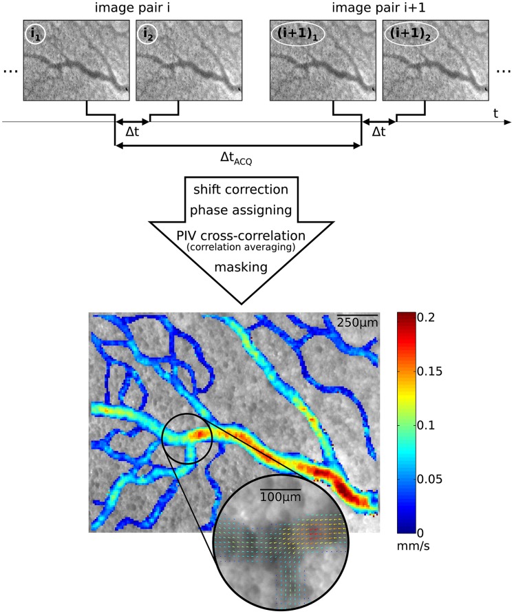
. A selection is enlarged to show the corresponding time-averaged velocity vector field, illustrating the spatial resolution of the measurement results.
Figure 5
Figure 5. Time-averaged velocity magnitudes of a measurement region are shown, together with with the corresponding skeleton (black line), branch points (white circles), and end points (gray circles).
The flow enters the measurement region from the right. Note that a non-linear color scale was used for the velocity magnitude.
Figure 6
Figure 6. Multiple parabolic fits at several locations on the vessel centerline were performed to obtain a single characteristic velocity and diameter for each vessel segment.
The time-averaged flow rate is assumed constant throughout the vessel segment. The valid region is bounded by 0.5 and 1.5×the median flow rate, and the red-encircled data points were not incorporated, due to a strongly deviating flow rate. Note that the fitted diameters and flow rates for the two data points on the far right are too large to be visible in the graph.
Figure 7
Figure 7. Schematic diagrams of studied structural parameters are shown for clarity.
These parameters are: the tortuosity formula image
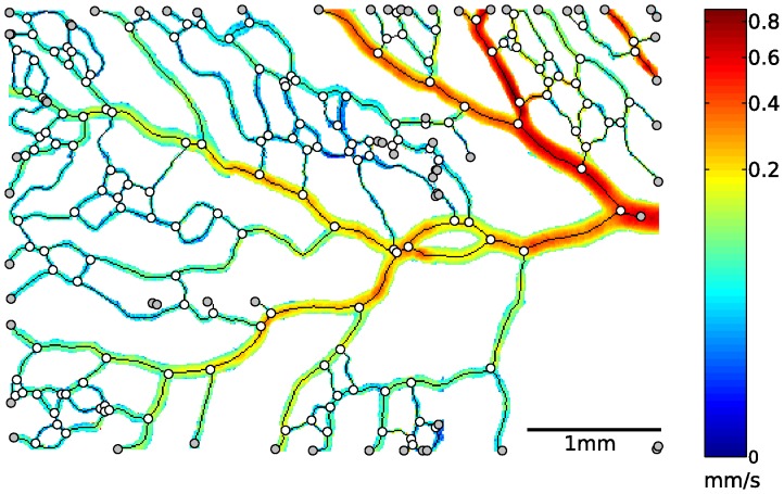
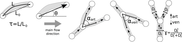
, the angle between the vessel segment and the main flow direction formula image, the arterial branching angle formula image, the venous branching angle formula image, and Murray’s law ratio for both arterial and venous branches formula image and formula image.
Figure 8
Figure 8. Networks are modeled as a collection of connected vessel segments, here shown with corresponding diameter and color-coded time-averaged mean velocity for two consecutive measurements T1(a) and T2(b).
Besides a general velocity increase, the part of the network in the upper right corner seems to have become responsible for a larger part of the total blood flow in this region (see also text). The flow enters the measurement region from the right. Note the two different non-linear color scales for (a) and (b).
Figure 9
Figure 9. The variety in time-averaged mean velocities for all vessel segment diameters are shown for two consecutive measurements T1 and T2.
For three vessel segments (I, II, and III, indicated in Figure 8), the changes in diameter and time-averaged velocity from T1 tot T2 are indicated by the dashed arrows. The cross-sectional velocity profiles shown for three data points (A, B, and C, indicated in Figure 8) show consistency despite the different time-averaged velocities.
Figure 10
Figure 10. The bar chart shows the probability density function of the relative flow balance for embryo 3, at T2.
This can be represented by a normal distribution which should ideally have a mean formula image 
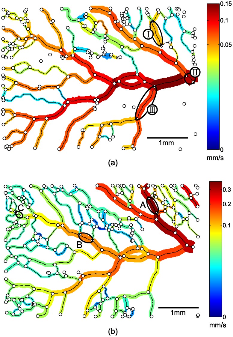
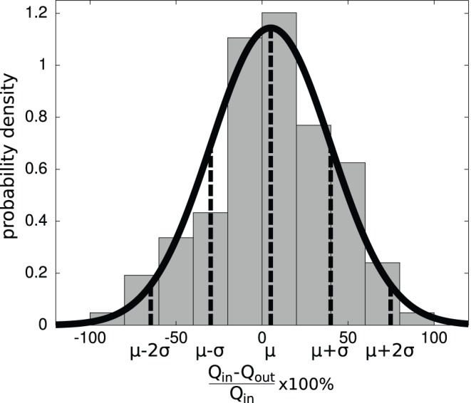
close to zero and a small standard deviation formula image.

Similar articles

Cited by

References

    1. Chapman W (1918) The effect of the heart-beat upon the development of the vascular system in the chick. Am J Anat 23: 175–203.
    1. Le Noble F, Moyon D, Pardanaud L, Yuan L, Djonov V, et al. (2004) Flow regulates arterial-venous differentiation in the chick embryo yolk sac. Dev 131: 361–375. - PubMed
    1. Lucitti J, Jones E, Huang C, Chen J, Fraser S, et al. (2007) Vascular remodeling of the mouse yolk sac requires hemodynamic force. Dev 134: 3317–3326. - PMC - PubMed
    1. Pries A, Secomb T (2010) Modeling structural adaptation of microcirculation. Microcirc 15: 753–764. - PMC - PubMed
    1. Nguyen T, Eichmann A, Le Noble F, Fleury V (2006) Dynamics of vascular branching morphogenesis: the effect of blood and tissue flow. Phys Rev E 73: 061907. - PubMed

Publication types