Spatiotemporal receptive fields of barrel cortex revealed by reverse correlation of synaptic input

Abstract

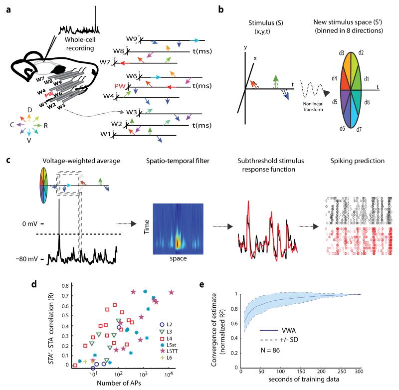
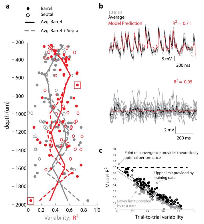
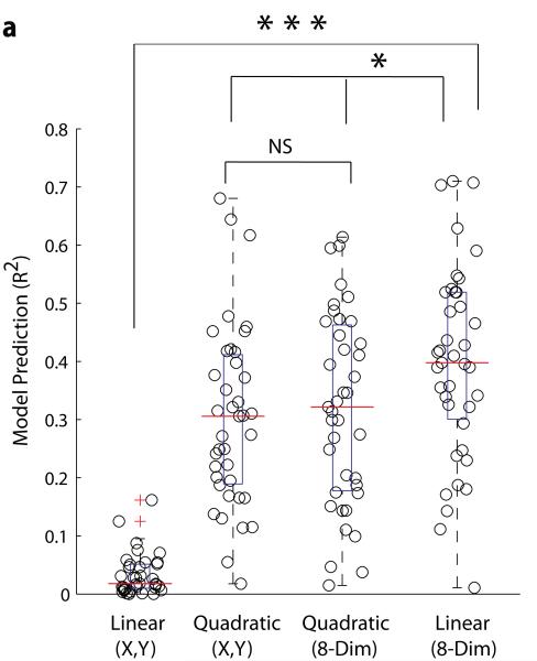
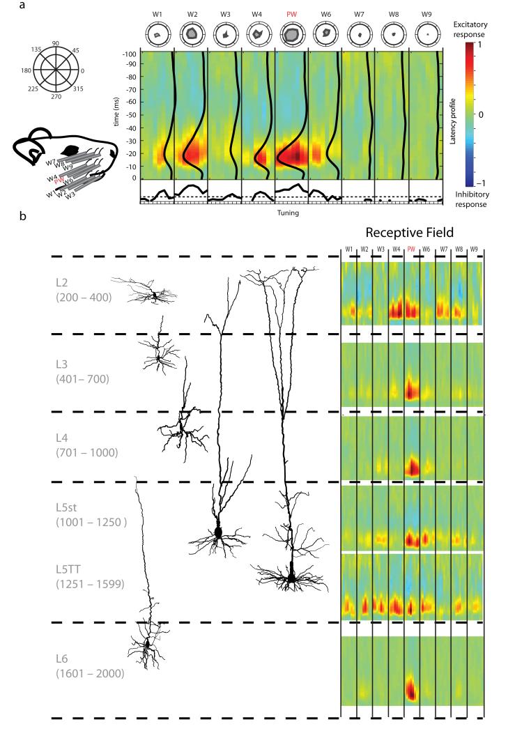
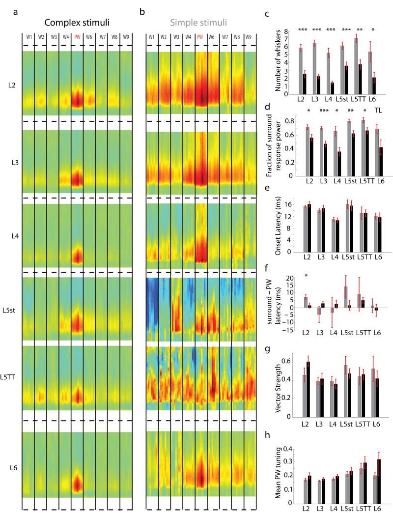
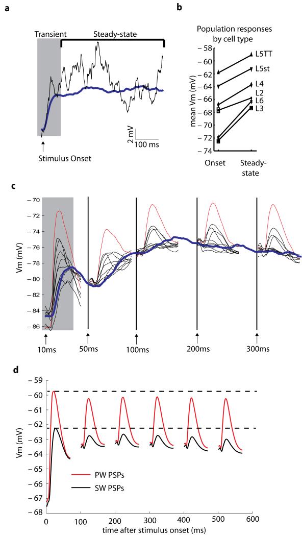
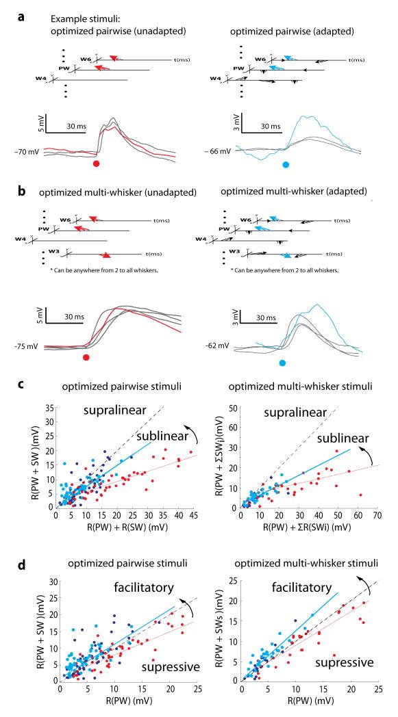
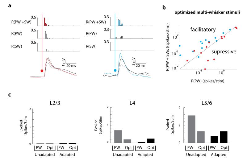
Of all of the sensory areas, barrel cortex is among the best understood in terms of circuitry, yet least understood in terms of sensory function. We combined intracellular recording in rats with a multi-directional, multi-whisker stimulator system to estimate receptive fields by reverse correlation of stimuli to synaptic inputs. Spatiotemporal receptive fields were identified orders of magnitude faster than by conventional spike-based approaches, even for neurons with little spiking activity. Given a suitable stimulus representation, a linear model captured the stimulus-response relationship for all neurons with high accuracy. In contrast with conventional single-whisker stimuli, complex stimuli revealed markedly sharpened receptive fields, largely as a result of adaptation. This phenomenon allowed the surround to facilitate rather than to suppress responses to the principal whisker. Optimized stimuli enhanced firing in layers 4-6, but not in layers 2/3, which remained sparsely active. Surround facilitation through adaptation may be required for discriminating complex shapes and textures during natural sensing.

Figure 1. Reverse correlation of intracellular recordings can rapidly and accurately identify spatiotemporal receptive fields (STRFs)

a, Schematic of the experimental setup. Left, barrel cortex neurons were recorded intracellularly during complex multi-whisker stimulation (sparse noise) to 9 whiskers. Right, schematic of complex multi-whisker stimulation. Arrows represent independent deflections of 9 whiskers. Deflections occur stochastically in time and direction (any of 360°). b, Nonlinear stimulus representation. Whisker movements are represented in an 8 angle-binned space instead of Cartesian space. c, The voltage-weighted average (VWA) of stimulus patterns estimates the spatiotemporal filter (K) for an individual neuron. The accuracy of the spatiotemporal filter is tested by predicting the response of the neuron to novel stimuli (cross-validation). The filter accurately predicts both the subthreshold response of the neuron as well as the spiking response. d, The relationship between the VWA and the STA is plotted as the correlation coefficient (R) between the predicted STA (STA’) and the true spike-triggered average (STA). The STA’ is the prediction calculated using the VWA and the appropriate noisy-threshold operation. As the number of spikes used for STA estimation increases, the mean correlation between the STA’ and STA becomes stronger, irrespective of laminar location or cell type of the recorded neuron. e, The speed of convergence for the VWA as a function of the amount of amount of data (seconds) used to train the model. The plot is on population data, dashed lines and shaded areas represent ± 1 SD.

Figure 2. Linearized model captures a majority of the predictable synaptic input for neurons in all layers of S1

a, Depth dependent relationship of the model performance and neural variability. Model performance (red) – defined as the cross-validated prediction of the VWA on trial averaged responses; – and neural variability (grey) – defined as the trial-to-trial variability between repeated presentations of identical stimuli, are plotted as a function of recording depth for each neuron. There is an inverse relationship between the model performance and neural variability in all neurons and layers. b, Responses of a neuron to ten repetitions of the same stimulus (gray traces) to illustrate neural variability along with the average response (blue) and predicted response (red). The two examples correspond to the data points inside red boxes in 2A, and represent examples of neurons with high prediction quality and low variability (top) and low prediction quality and high variability (bottom). c, The model performance (R²) tested on single-trial responses using training data (black) and cross-validation/test data (grey) is plotted against the trial-to-trial variability for each neuron. Convergence of the test-performance and training-performance at zero variability between an R² of 0.64 and 0.68.

Figure 3. Comparison of models

a, In order to verify the superiority of the stimulus-transformed linear model over other linear and nonlinear models (quadratic regression), we compared the performance of these different models on a subset of neurons (N=39). For the four models, calculated either in the (x,y) space or the 8 dimensional stimulus transformed space (8-dim) we show jitterplots and boxplots of the cross-validated prediction, R². The red line indicates median values. The linear model in the (x,y) space had an R² 0.0340 ± 0.0362 and a median value of 0.0179, and performed significantly worse than the linear model in the 8-Dim representation (p-value < 0.001, t-test). The quadratic regression in the (x,y) space had an R² 0.303 ± 0.155 and a median value of 0.306. The quadratic regression in the 8-Dim representation had an average R² of 0.319 ± 0.165, a median value of 0.322, and did not perform significantly better than the quadratic regression in the (x,y) space (p-value = 0.65, t-test). The linear model in the 8-Dim representation performed significantly better than the quadratic (x,y) and the quadratic 8-Dim (p-values = 0.0113, 0.0416 respectively; t-test) and had an average R² of 0.397 ± 0.167.

Figure 4. Example whisker spatiotemporal receptive fields (STRFs) for morphologically identified cells across layers

a, Left top, the pinwheel corresponds to 8 angle bins used to represent the tuning of the individual whiskers. Left bottom, schematic of the 9 whisker stimulators arranged on the rat’s face with the PW in the center and 8 SWs. Middle, a representative STRF for a layer 5 slender tufted (L5st) neuron. Each whisker contains 8 columns corresponding to movement in one of the 8 angle bins. Collapsing over time reveals the angular tuning for each whisker (bottom, dashed lines represent 99% significance) and is equivalent to unwrapping the polar plots of the same data (top). Collapsing over space reveals the average latency of response for each neuron, illustrated by the 9 black vertical curves overlying the STRF. b, Example STRFs for morphologically identified and reconstructed neurons from each layer.

Figure 5. Complex stimuli reveal dramatically sharpened receptive fields relative to conventional stimuli

Population averaged STRFs were calculated for neurons of the same cell type. a, Population STRFs based on complex multi-whisker stimuli. b, Population STRFs simple single-whisker stimulation for the same neurons as in A. c – h, Receptive field properties for complex (black) versus simple (gray) stimuli (* p < 0.05; ** p < 0.01; *** p < 0.001; TL, p < 0.1; all tests were non-parametric two sided rank-sum test). Bars, means ± SEM. c, Adapted STRFs had significantly fewer responsive whiskers than unadapted STRFs. d, For adapted STRFs the total fraction of the response power contained in the surround receptive field was significantly less than in unadapted neurons. e, Onset latency of the receptive field (usually, but not always, the onset of the PW response) was unchanged between groups. f, The average latency between the onset of the PW response and the mean onset of the SW responses was shortened for adapted STRFs, and was significant in L2 (p<0.05, t-test). g, The vector strength, a measure of coherence or directional similarity between significantly responsive whiskers, was highest in infra and supra-granular layers but was unchanged between simple stimuli and complex stimuli (0 anti-coherent, 1 perfectly coherent). h, Directional tuning of the PW, defined as strength of response to the preferred direction divided by the summed response to all directions, was always higher during complex stimuli but results were not significant (0.125 = no tuning preference; 1.0 = tuned to a single direction).

Figure 6. Neural adaptation underlying receptive field changes

a, The trial averaged response of a neuron over 300 unique trials of complex stimulus (blue) and the response to a single trial (black) reveals a strong stimulus transient and tonic depolarization that is dependent on stimulus onset. b, Comparison of the mean V_m at stimulus onset and during steady-state response reveals a tonic depolarization of 1-5 mV for each cell type and layer. c, The response to PW deflections (red) and the eight SW deflections (black) depends on the state of the neuron and/or circuit. The average PW and SW deflections were measured during the five epochs indicated by the arrows. The trial averaged response is shown in blue. d, For all neurons (N = 86), the average PSP amplitude and peak V_m for PW and the average for the eight SWs (as in C) are plotted in time. Peak potentials for the PW (red) and SWs (black) remain relatively invariant and the main factor affecting PSP size is the tonic depolarization of membrane potential during adaptation.

Figure 7. Adaptation linearizes summation of synaptic inputs and allows surrounds to facilitate rather than suppress responses

a, The best pairwise stimulus for each neuron was determined from the VWA and played back in isolation (unadapted, left) or embedded within random surround stimuli (adapted, right). Black, trial-averaged responses of a neuron to each of the two whiskers, R(PW) or R(SW). Circles, stimulus onset. The pairwise deflection, R(PW+SW), is shown in red (unadapted) or cyan (adapted). b, same as in panel a but for the best multi-whisker stimuli (2-9 whiskers). c, For all neurons (N = 46 unadapted in red; N = 75 adapted in blue/cyan) response to the pairwise deflection R(PW+SW) was plotted against the sum of responses to individual deflections R(PW)+R(SW). Cyan points represent neurons observed during both adapted and unadapted conditions and therefore have a red counterpart. Blue points represent neurons observed only during adaptation. Pairwise summation is nearly linear during adaptation (blue and cyan) (slope 0.723, r 0.506, p < 10⁻⁸) and sub-linear under unadapted conditions (red) (slope 0.346, r 0.738, p < 10⁻⁹). Similar behavior was observed for the optimal multi-whisker stimuli (right) (N=33 unadapted, 36 adapted; 33 matched pairs) (adapted: slope 0.491, r 0.631, p < 10⁻⁷; unadapted: slope 0.223, r 0.442, p < 10⁻⁹). d, For the same data as in c responses to pairwise deflections [R(PW+SW)] were compared to responses to the PW deflections alone [R(PW)]. Surround inputs facilitated the PW response during adaptation but suppressed the PW response without adaptation.

Figure 8. Spiking responses are facilitated by the surround in adapted neurons yet spiking remains sparse in superficial layers

a, Examples of spiking neurons during the delivery of optimal stimuli in unadapted neurons (left) and adapted neurons (right). b, Surround inputs facilitate the PW response in adapted neurons but suppress the PW response in unadapted neurons (p = 0.02, 0.30, respectively; two-sided sign test). c, Evoked spiking activity in adapted and unadapted neurons demonstrates that the PW alone is the most effective driver of spiking activity in unadapted neurons but optimal multi-whisker stimuli are more effective in adapted neurons.

References

1. Brecht M, Roth A, Sakmann B. Dynamic receptive fields of reconstructed pyramidal cells in layers 3 and 2 of rat somatosensory barrel cortex. J Physiol. 2003;553:243–265. - PMC - PubMed
1. Manns ID, Sakmann B, Brecht M. Sub- and suprathreshold receptive field properties of pyramidal neurones in layers 5A and 5B of rat somatosensory barrel cortex. J Physiol. 2004;556:601–622. - PMC - PubMed
1. Moore CI, Nelson SB. Spatio-temporal subthreshold receptive fields in the vibrissa representation of rat primary somatosensory cortex. J Neurophysiol. 1998;80:2882–2892. - PubMed
1. Zhu JJ, Connors BW. Intrinsic firing patterns and whisker-evoked synaptic responses of neurons in the rat barrel cortex. J Neurophysiol. 1999;81:1171–1183. - PubMed
1. de Kock CP, Bruno RM, Spors H, Sakmann B. Layer- and cell-type-specific suprathreshold stimulus representation in rat primary somatosensory cortex. J Physiol. 2007;581:139–154. - PMC - PubMed
Publication types
LinkOut - more resources