Using the power balance model to simulate cross-country skiing on varying terrain

Abstract

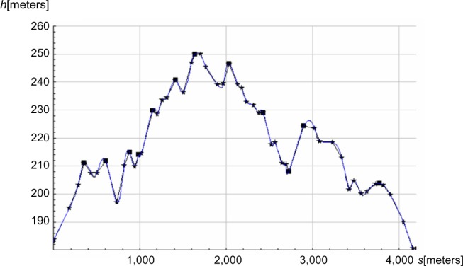
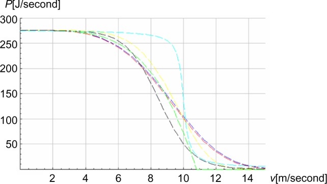
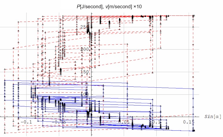
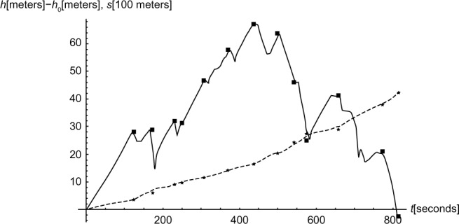
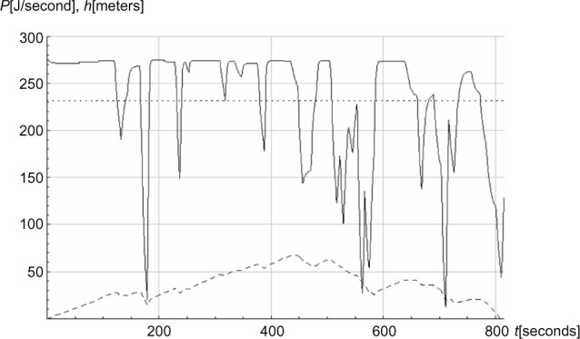
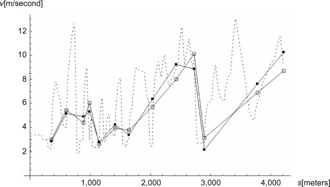
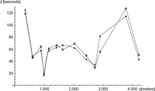
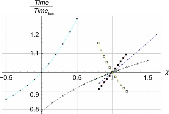
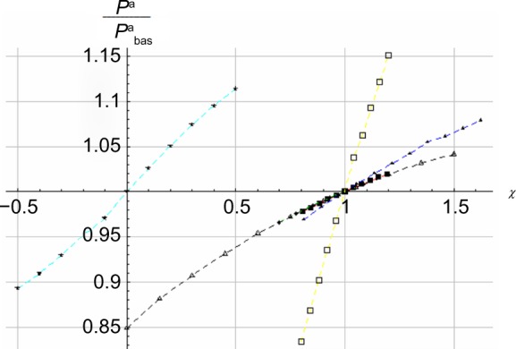
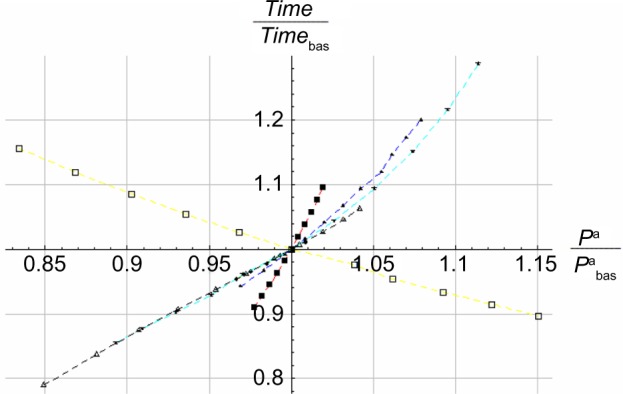
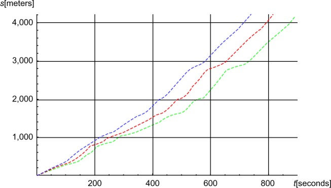
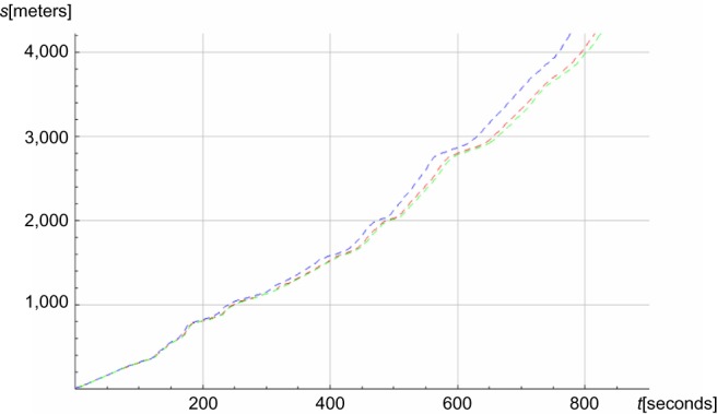
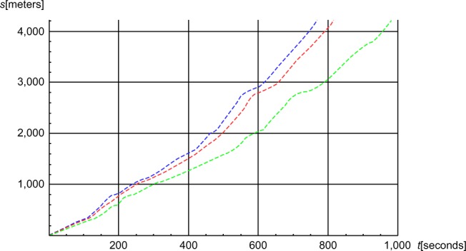
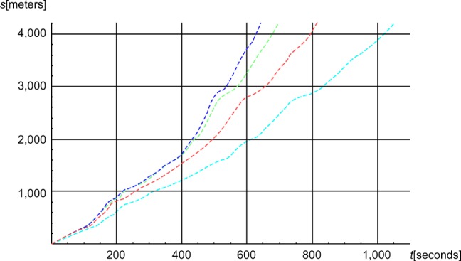
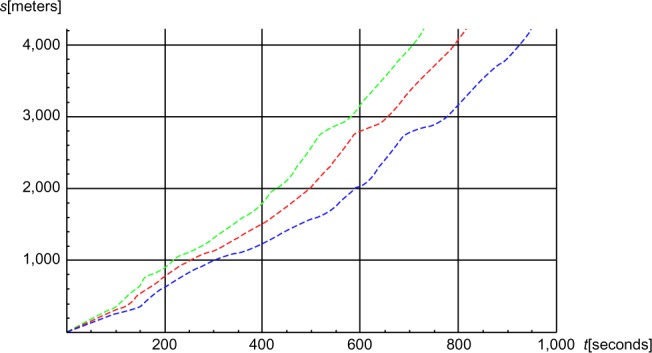
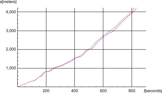
The current study adapts the power balance model to simulate cross-country skiing on varying terrain. We assumed that the skier's locomotive power at a self-chosen pace is a function of speed, which is impacted by friction, incline, air drag, and mass. An elite male skier's position along the track during ski skating was simulated and compared with his experimental data. As input values in the model, air drag and friction were estimated from the literature based on the skier's mass, snow conditions, and speed. We regard the fit as good, since the difference in racing time between simulations and measurements was 2 seconds of the 815 seconds racing time, with acceptable fit both in uphill and downhill terrain. Using this model, we estimated the influence of changes in various factors such as air drag, friction, and body mass on performance. In conclusion, the power balance model with locomotive power as a function of speed was found to be a valid tool for analyzing performance in cross-country skiing.

Keywords: air drag; efficiency; friction coefficient; locomotive power; speed.

Figure 1

The height (h) in the terrain as a function of accumulated distance (s). Notes: Straight lines are drawn between each star, which means a piecewise linear track; ■ denotes 13 points where time measurements were made; blue curve is a cubic spline fit.

Figure 2

The locomotive power (P) as a function of speed (v) for the three models for various parameter values. Notes: Blue, model 1 (n=4, b=10.1 m/s); red, model 1 (n=4, b=10.0 m/s); yellow, model 1 (n=6, b=10.0 m/s); green: model 2 (n=4, b=10.8 m/s); black, model 3 (a=8.5 m/s, b=1.0 m/s); cyan, function from Sundstrøm et al scaled vertically to reach maximum P_max=275 when v=0.

Figure 3

Blue: Locomotive power (P) versus inclination sin(α). Red: Speed (v) ×10 versus inclination sin(α).

Figure 4

The experimental height (h−h₀) and accumulated distance (s), and simulated height (h−h₀) and accumulated simulated distance (s) as functions of time (t) in seconds. Notes: h₀ =183 m is initial height. ■ denotes 13 points where time measurements were made for height. The height is relative to initial height in meters; ★denotes 13 points where time measurements were made for accumulated distance. The distance is in units of 100 m; — denotes simulated height (h−h₀); ------ denotes accumulated simulated distance (s).

Figure 5

The locomotive power (P) and height (h) of the racing track as functions of time (t) in seconds. Notes: _____ denotes P(t); -------- denotes average P(t); - - - - - denotes track profile h(t).

Figure 6

The experimental and simulated average speed, and the simulated speed as functions of accumulated distance (s). Notes: ■ denotes experimental average speed in m/second; □ denotes simulated average speed in m/second; .... denotes simulated speed in m/second.

Figure 7

The experimental and simulated time difference (δt) between the points where time measurements were made, as functions of accumulated distance (s). Notes: ★ denotes experimental time difference between two subsequent points; ✩ denotes simulated time difference between two subsequent points.

Figure 8

The relative time to complete the race as a function of the proportion χ of the baseline values for m, μ, ρ, V, P_max, and C_dA. Notes: ■ Red, mass; ▲ blue, friction; ♦ green, density; ★ cyan, wind speed; □ yellow, maximum locomotive power; △ black, drag.

Figure 9

The relative locomotive power $(P^{\text{a}}/P_{\text{bas}}^{\text{a}})$ as a function of the the proportion χ of the baseline values for m, μ, ρ, V, P_max, and C_dA. Notes: ■ Red, mass; ▲ blue, friction; ♦ green, density; ★ cyan, wind speed; □ yellow, maximum locomotive power; △ black, drag.

Figure 10

The relative time to complete the race as a function of the relative locomotive power. Notes: ■ Red, mass; ▲ blue, friction; ♦ green, density; ★ cyan, wind speed; □ yellow, maximum locomotive power; △ black, drag.

Figure 11

The accumulated simulated distance (s) in meters as functions of time (t) in seconds. Notes: Red, baseline; blue, m =62.5 kg; green, m =92.5 kg (where m is body mass).

Figure 12

The accumulated simulated distance (s) in meters as functions of time (t) in seconds. Notes: Red, baseline; blue, ρ =0.90 g/cm³; green, ρ =1.40 g/cm³ (where ρ is air density).

Figure 13

The accumulated simulated distance (s) in meters as functions of time (t) in seconds. Notes: Red, baseline; blue, μ =0.03; green, μ =0.06 (where μ is the friction coefficient).

Figure 14

The accumulated simulated distance (s) in meters as functions of time (t) in seconds. Notes: Red, baseline; blue, C_dA =0; green, −5 m/second tailwind; cyan, +5 m/second headwind (where C_d is the drag coefficient, and A is the projected front area of the skier).

Figure 15

The accumulated simulated distance (s) in meters as functions of time (t) in seconds. Notes: Red, baseline; blue, P_max =220 J/second; green, P_max =330 J/second (where P_max is maximum locomotive power).

Figure 16

The accumulated simulated distance (s) in meters as functions of time (t) in seconds. Notes: Red, baseline; blue, cubic spline.

References

-
- Bergh U, Forsberg A. Influence of body mass on cross-country ski racing performance. Med Sci Sports Exerc. 1992;24(9):1033–1039. - PubMed
- Norman RW, Komi PV. Mechanical energetics of world-class cross-country skiing. Int J Sport Biomech. 1987;3:353–369.
- Smith GA. Biomechanical analysis of cross-country skiing techniques. Med Sci Sports Exerc. 1992;24(9):1015–1022. - PubMed
- Sandbakk O, Ettema G, Holmberg HC. The influence of incline and speed on work rate, gross efficiency and kinematics of roller ski skating. Eur J Appl Physiol. 2012;112(8):2829–2838. - PubMed
LinkOut - more resources
Full Text Sources
Other Literature Sources
Research Materials