An experimental limit on the charge of antihydrogen

Abstract

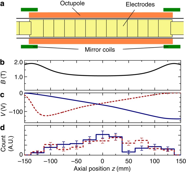
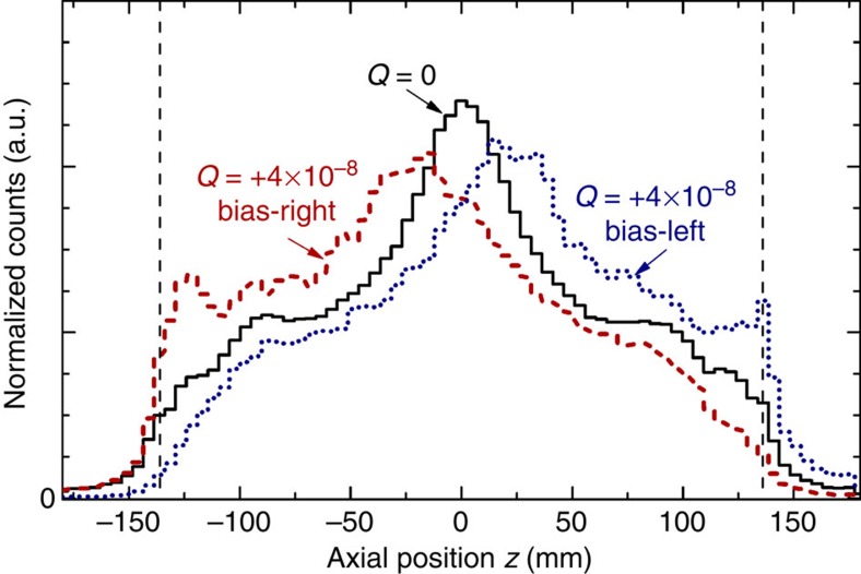
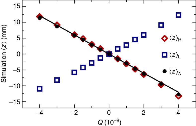
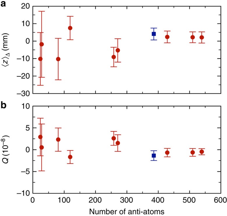
The properties of antihydrogen are expected to be identical to those of hydrogen, and any differences would constitute a profound challenge to the fundamental theories of physics. The most commonly discussed antiatom-based tests of these theories are searches for antihydrogen-hydrogen spectral differences (tests of CPT (charge-parity-time) invariance) or gravitational differences (tests of the weak equivalence principle). Here we, the ALPHA Collaboration, report a different and somewhat unusual test of CPT and of quantum anomaly cancellation. A retrospective analysis of the influence of electric fields on antihydrogen atoms released from the ALPHA trap finds a mean axial deflection of 4.1 ± 3.4 mm for an average axial electric field of 0.51 V mm(-1). Combined with extensive numerical modelling, this measurement leads to a bound on the charge Qe of antihydrogen of Q=(-1.3 ± 1.1 ± 0.4) × 10(-8). Here, e is the unit charge, and the errors are from statistics and systematic effects.

Figure 1. Experimental summary.

(a) A schematic of the antihydrogen production and trapping region of the ALPHA apparatus, showing the cryogenically cooled cylindrical Penning–Malmberg trap electrodes, and the mirror and octupole magnet coils. Our positron source (not shown) is towards the right, and the antiproton decelerator (not shown) is towards the left. (b) The on-axis magnetic field B as a function of z. (c) The on-axis electrostatic potentials V used to establish the Bias-Right (red dashed line) and Bias-Left (blue solid line) configurations. (d) Normalized histograms of the experimental z positions of the annihilations in the Bias-Right (red dashed line) and Bias-Left (blue solid line) configurations. The error bars show the expected deviation of the distribution based on the number of observed antiatoms in each bin.

Figure 2. Simulated annihilation z-distributions.

Three simulated annihilation z-distributions, for antiatoms with Q=0 (black solid line) and Q=+4 × 10⁻⁸ under Bias-Right (red dashed line) and Bias-Left (blue dotted line) conditions. The vertical dashed lines indicate the locations of the cuts at z= ±136 mm.

Figure 3. Simulated dependence of the axial shifts on Q.

The average annihilation locations ‹z› in the Bias-Right (red diamonds) and Bias-Left (blue squares) configurations, as well as the resulting ‹z›_Δ (black dots), as found in the simulations with detector efficiency and resolution corrections. The statistical error of ±0.1 mm in the calculated values of ‹z›_R and ‹z›_L, and ±0.07 mm for ‹z›_Δ, is too small to be shown with clarity. The black solid line is the least-squares linear fit that best describes the variation of ‹z›_Δ with Q. The fit is constrained to pass through ‹z›_Δ=0 at Q=0, consistent with the simulations to within statistical uncertainty and with our expectation that the bias electric fields have no effect on particles for which Q=0.

Figure 4. Measured and simulated antihydrogen cumulative distribution function.

The simulated time-reversed cumulative distribution function (CDF) of the time of annihilation for the nominal, Maxwellian distribution (solid red), uniform (short dashed green) distribution and linear (long dashed orange) distribution. The inset figure depicts the candidate energy distributions f(E). The Maxwellian distribution is a much better match to both the 2010 (solid dark blue) experimental data and the 2011 (dashed light blue) experimental data than either the Uniform or Linear distributions. The error bars show the expected deviation of the CDF based on the number of observed antiatoms used to compute the CDF at each time.

Figure 5. Data selection.

The ‹z›_Δ and Q plotted as a function of the number of antiatoms included in the analysis for the data in Table 3. The principle case is the blue square point. Note that the data are generally, but not always, cumulative with increasing number of antiatoms. Thus, the points are not generally independent. Also note that the sensitivity, s, used to scale from ‹z›_Δ to Q varies from −3.31 × 10⁻⁹mm⁻¹ (Principle data set) to −0.224 × 10⁻⁹mm⁻¹ (no z cut data sets). In a, the error bars show the s.e. values of the mean in ‹z›_Δ, and in b, these errors scaled by the sensitivity s.

References

1. Amoretti M. et al. Production and detection of cold antihydrogen atoms. Nature 419, 456–459 (2002). - PubMed
1. Gabrielse G. et al. Background-free observation of cold antihydrogen and a field-ionization analysis of its states. Phys. Rev. Lett. 89, 213401 (2002). - PubMed
1. Enomoto Y. et al. Synthesis of cold antihydrogen in a cusp trap. Phys. Rev. Lett. 105, 243401 (2010). - PubMed
1. Andresen G. B. et al. Trapped antihydrogen. Nature 468, 673–676 (2010). - PubMed
1. Andresen G. B. et al. Confinement of antihydrogen for 1000 seconds. Nat. Phys. 7, 558–564 (2011).
Publication types