Perception and coding of high-frequency spectral notches: potential implications for sound localization

Abstract

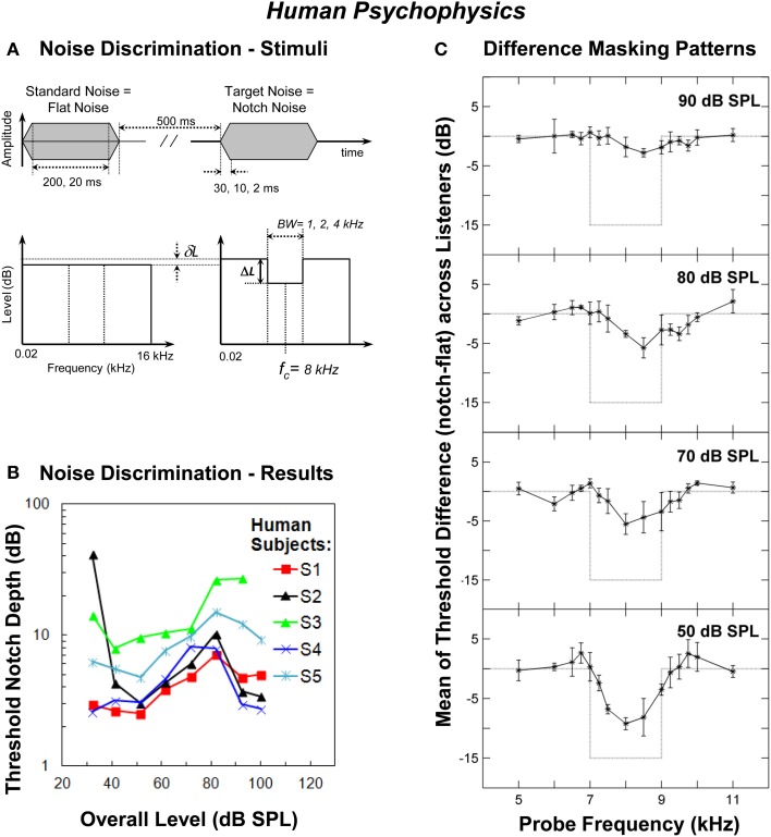
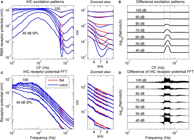
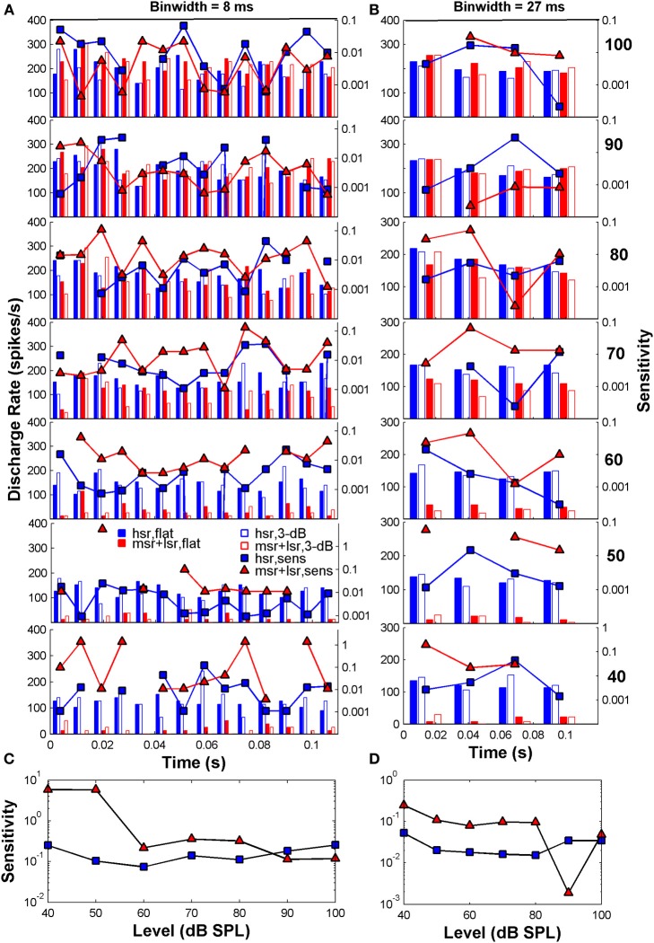
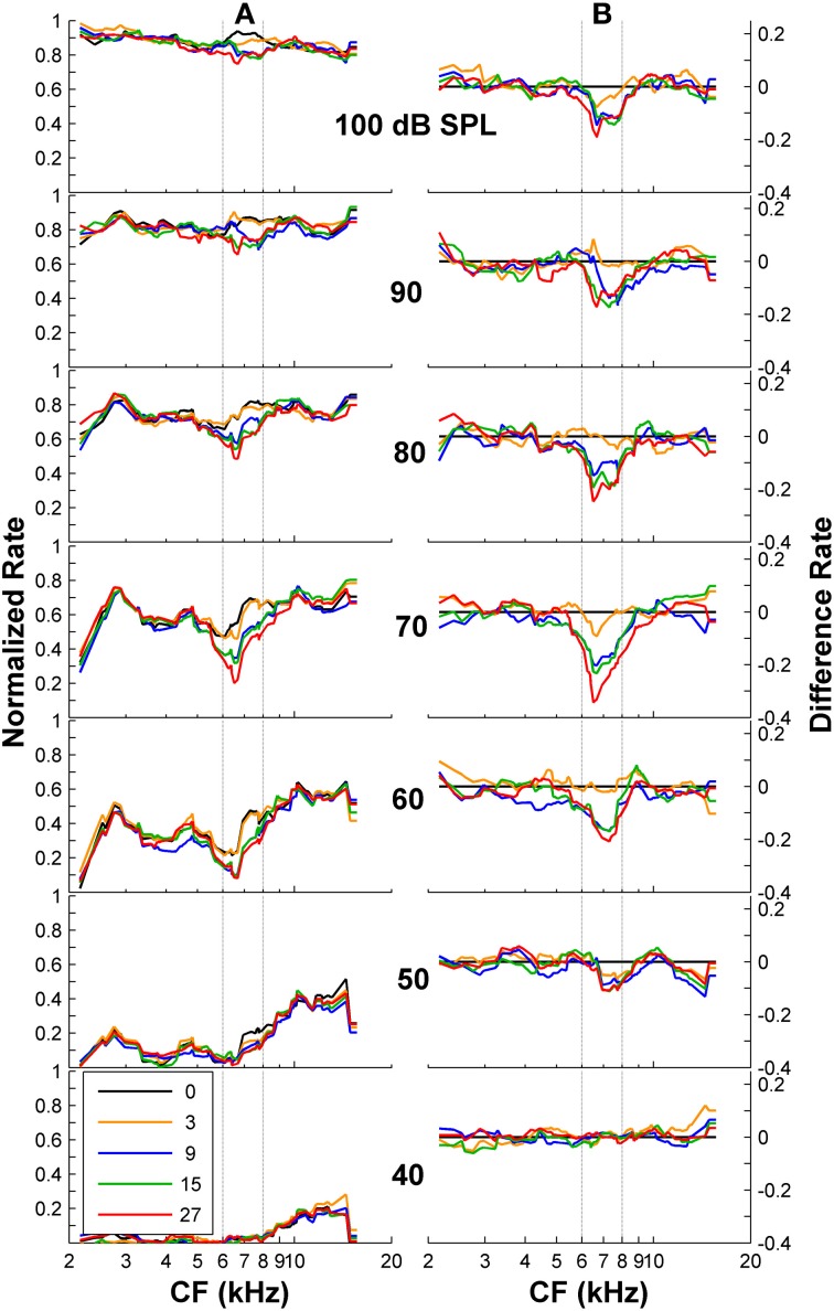
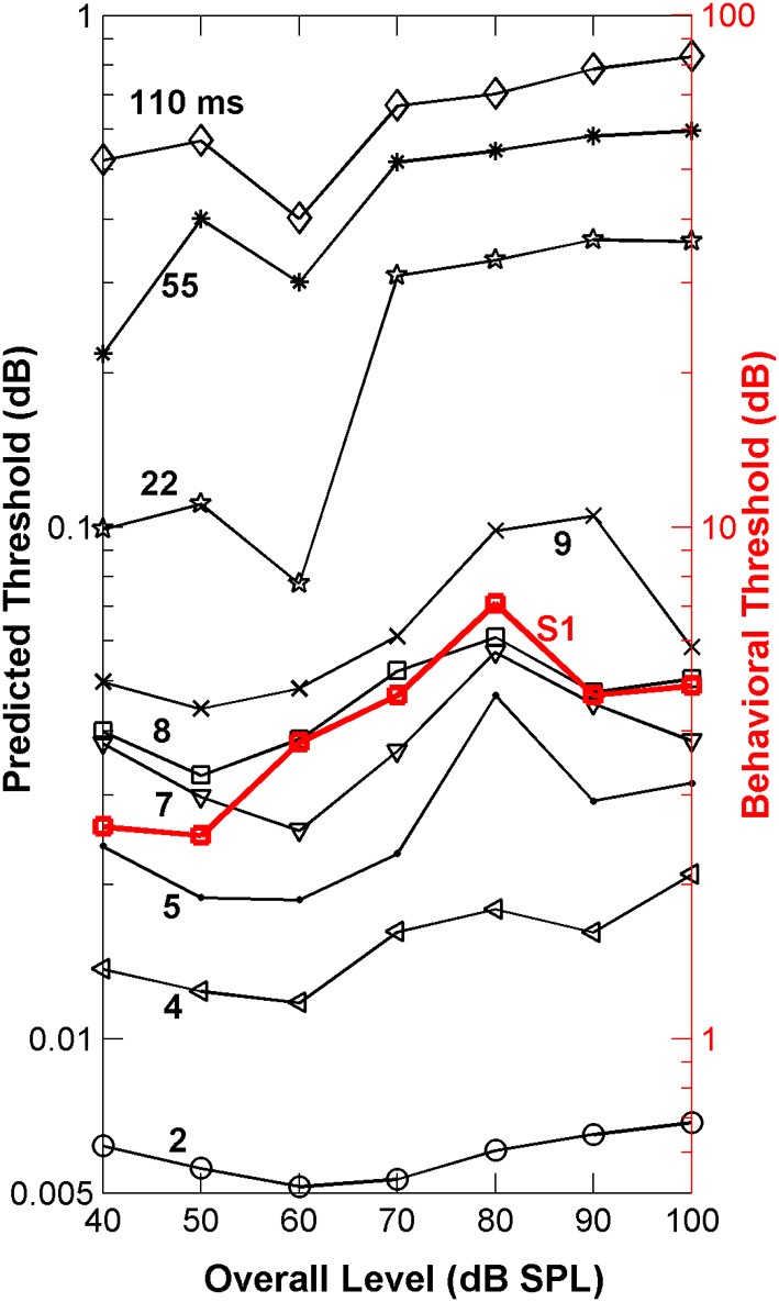
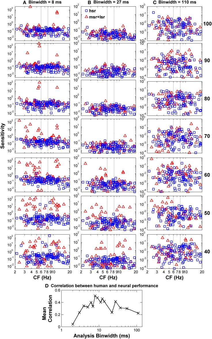
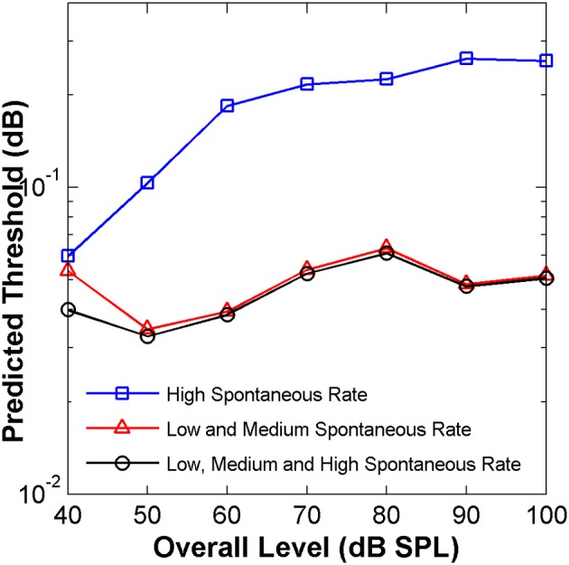
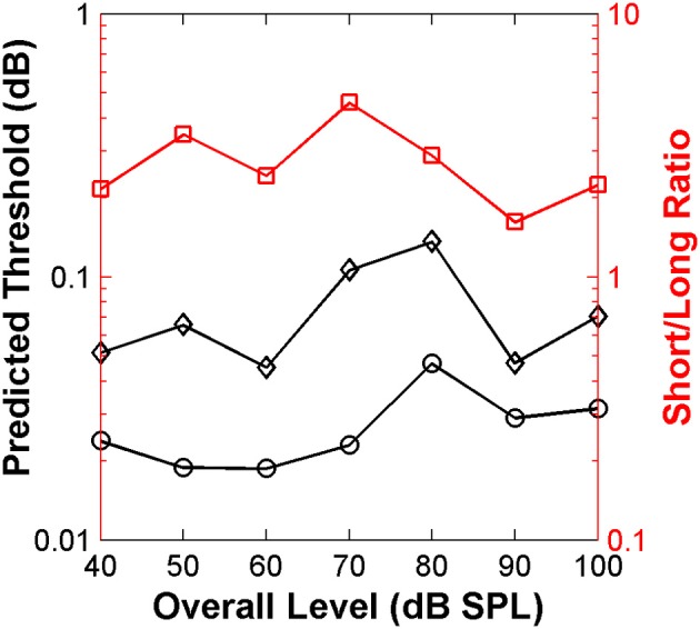
The interaction of sound waves with the human pinna introduces high-frequency notches (5-10 kHz) in the stimulus spectrum that are thought to be useful for vertical sound localization. A common view is that these notches are encoded as rate profiles in the auditory nerve (AN). Here, we review previously published psychoacoustical evidence in humans and computer-model simulations of inner hair cell responses to noises with and without high-frequency spectral notches that dispute this view. We also present new recordings from guinea pig AN and "ideal observer" analyses of these recordings that suggest that discrimination between noises with and without high-frequency spectral notches is probably based on the information carried in the temporal pattern of AN discharges. The exact nature of the neural code involved remains nevertheless uncertain: computer model simulations suggest that high-frequency spectral notches are encoded in spike timing patterns that may be operant in the 4-7 kHz frequency regime, while "ideal observer" analysis of experimental neural responses suggest that an effective cue for high-frequency spectral discrimination may be based on sampling rates of spike arrivals of AN fibers using non-overlapping time binwidths of between 4 and 9 ms. Neural responses show that sensitivity to high-frequency notches is greatest for fibers with low and medium spontaneous rates than for fibers with high spontaneous rates. Based on this evidence, we conjecture that inter-subject variability at high-frequency spectral notch detection and, consequently, at vertical sound localization may partly reflect individual differences in the available number of functional medium- and low-spontaneous-rate fibers.

Keywords: HRTF; auditory nerve; head-related transfer function; phase-locking; rate profile; temporal profile.

Figure 1

Human psychophysics. (A) Schematic description of the waveforms and spectra of the flat-spectrum (“Standard Noise”) and notch (“Target Noise”) noises used in the noise discrimination experiment. The notch depth (ΔL) was defined as the difference in dB between the spectrum level in the notch and the reference spectrum level of the noise in the notch side bands. δL represents the reduction in spectrum level applied to the standard noise in order to make its overall level equal to that of the target noise. Also indicated are the values of stimulus duration, stimulus on/off time and the notch bandwidth (BW) tested in the experiments (adapted from Alves-Pinto and Lopez-Poveda, 2005). (B) Individual threshold notch depths for discriminating between the standard and target noises (panel A) as a function of overall stimulus level. The notch bandwidth was 2 kHz and the notch depth is in dB re the spectrum level in the notch side bands. Each symbol/color illustrates the results for a different listener (adapted from Alves-Pinto and Lopez-Poveda, 2005). (C) Differences between the masking patterns of the flat-spectrum and notch noise (notch—flat) at increasing masker levels averaged across listeners. Each panel illustrates the results for a different masker level, as indicated in the top-right corner of the panel. Error bars represent one standard deviation from the mean difference. Dotted lines illustrate the difference between the spectra of the two noises (adapted from Figure 8 of Alves-Pinto and Lopez-Poveda, 2008).

Figure 2

Computational simulation of inner hair cell receptor potentials. Simulated IHC responses to broadband noises with a flat spectrum and with a 2-kHz wide, 15-dB spectral notch centered at 7 kHz. The noise duration was longer than that used in the psychoacoustical experiments (0.5 vs. 0.2 s) to obtain “smoother” responses. (A) IHC excitation pattern representation of the flat-spectrum (red) and notch noises (blue). Each curve illustrates the average (rms) receptor potential of each IHC as a function of the cell's CF, for a different stimulus level, from 40 to 100 dB SPL, as indicated by the numbers next to each trace. (B) Difference excitation patterns (in dB) normalized to the maximum value across CFs and intensities. The numbers next to each trace indicate stimulus intensity in dB SPL. (C) Spectra of the IHC receptor potential representation of the two noises for the same stimulus levels as in (A). Each curve depicts the frequency-wise summed spectra of individual IHC receptor potential spectra (see main text). (D) Difference receptor potential FFT (in dB) normalized to the maximum value across frequencies and intensities. In (B,D), the curves have been arbitrarily displaced vertically for convenience. Vertical dotted lines in (B,D) indicate the notch frequency band. The middle panels illustrate zoomed views of panels (A,C) over the frequency range of the spectral notch.

Figure 3

Auditory nerve data: example post-stimulus time histograms (PSTHs; scale on the left y-axis) and related sensitivity (scale on the right y-axis) for one HSR fiber (blue bars and squares: CF = 3.6 Hz, SR = 111 spikes/s, 10 repeats/stimulus) and one LSR fiber (red bars and triangles: CF = 6.9 Hz, SR = 11.2 spikes/s, 10 repeats/stimulus). (A) PSTHs calculated for time binwidths of 8 ms. (B) PSTHs calculated for a binwidth of 27 ms. In each panel, filled and open blue bars illustrate the PSTHs for the HSR fiber when stimulated with a flat-spectrum and 3-dB-deep notch noise, respectively. Filled and open red bars illustrate corresponding PSTHs for the LSR fiber. Each row illustrates results for a different stimulus level as indicated by the bold numbers on the right part of the figure (in dB SPL). Also represented in each panel is the fiber's sensitivity in each time bin (log-scale on the right y-axis) for each of the two fibers (blue squares for the HSR fiber; red triangles for the LSR fiber; one symbol per bin). Sensitivity was calculated using Equation (2b) and yields a measure of a fiber's ability to discriminate between the two stimuli through a change in the discharge rate evoked by them, in different time bins. Missing symbols indicate bins for which the two stimuli elicited identical discharge rates, hence sensitivity became zero. (C) Overall sensitivity as a function of stimulus level for each of the fibers represented in panel (A). Overall sensitivity for a given level was obtained by summing all the sensitivities across all bins for that level [Equation (2a)], represented by the symbols in the corresponding panel (A). Blue squares and red triangles illustrate the sensitivity vs. level function for the HSR and LSR fibers, respectively. (D) The same as in C but for time binwidths of 27 ms. Overall sensitivity for each fiber was obtained by summing all the sensitivities at the corresponding level in panel (B). The results presented in all panels are based on the responses of the same two AN fibers. For each fiber, different sensitivities within each time bin (panels A,B) produce different sensitivity vs. level functions (panels C,D).

Figure 4

Auditory nerve data: rate profiles for different overall noise levels and for different notch depths. (A) Normalized rate profiles. Each curve is for a different notch depth (in dB), as indicated by the inset. (B) Difference between the rate profiles for the flat-spectrum and the notched noises. The numbers in the inset denote notch depths in dB re spectrum level of the notch side bands. Vertical dashed lines illustrate the frequency band of the spectral notch.

Figure 5

Auditory nerve data: population d′ as a function of the noise overall level. The numbers in the inset indicate notch depths in dB re spectrum level of the notch side bands.

Figure 6

Auditory nerve data: psychoacoustically observed notch-depth thresholds vs. “ideal observer” predictions from neural data. Psychoacoustical (red squares, right ordinate axis) thresholds as a function of noise level for an example listener (S1; Figure 1B). Predicted thresholds (open symbols, left ordinate axis) were obtained using an “ideal observer” type of analysis of physiological AN responses [Equations (2a) and (2b)]. Different curves illustrate predicted thresholds when AN activity is analyzed over non-overlapping time binwidths of different durations, as indicated by the numbers next to each trace (in ms; adapted from Figure 1 of Lopez-Poveda et al., 2007).

Figure 7

Auditory nerve data: individual AN fiber sensitivity as a function of fiber's CF. Sensitivity values for HSR and LSR fibers are illustrated by blue squares and red triangles, respectively. Sensitivity was calculated for three different time binwidths: 8 ms (A), 27 ms (B), and 110 ms (C). Notice the different sensitivity scales used for the different binwidths. Stimulus level increases from the bottom to the top panel as indicated by the numbers on the right side of the figure (in units of dB SPL). Individual sensitivity values varied with stimulus level and with binwidth, with the highest sensitivity values occurring for different subgroups of fibers for different levels and binwidths. (D) Kendall's Tau non-parametric correlation between the shape of individual behavioral notch-depth thresholds (Figure 1B) and “ideal observer” neural predictions for different analysis time binwidths (black symbols in Figure 6). The figure illustrates the mean correlation coefficient values across five participants (Figure 1B).

Figure 8

Auditory nerve data: predicted threshold notch depth vs. level functions from an “ideal observer” analysis of neural responses from different fiber types, as indicated in the legend. Predictions are for an analysis time window of 8 ms.

Figure 9

Auditory nerve data: threshold notch depth vs. level functions predicted by an “ideal-observer” analysis of neural responses for noise bursts with different duration: 20 ms (diamonds) and 110 ms (circles). Red squares (right ordinate axis) illustrate the ratio between predicted thresholds for the long and short stimuli.

References

1. Alves-Pinto A., Lopez-Poveda E. A. (2005). Detection of high-frequency spectral notches as a function of level. J. Acoust. Soc. Am. 118, 2458–2469 10.1121/1.2032067 - DOI - PubMed
1. Alves-Pinto A., Lopez-Poveda E. A. (2008). Psychophysical assessment of the level-dependent representation of high-frequency spectral notches in the peripheral auditory system. J. Acoust. Soc. Am. 124, 409–421 10.1121/1.2920957 - DOI - PubMed
1. Alves-Pinto A., Lopez-Poveda E. A., Palmer A. R. (2005). Auditory nerve encoding of high-frequency spectral information, in Interplay Between Natural and Artificial Computation (IWINAC), eds Mira J., Álvarez J. R. (Berlin; Heidelberg: Springer-Verlag; ), 223–232
1. Ashmore J., Avan P., Brownell W. E., Dallos P., Dierkes K., Fettiplace R., et al. (2010). The remarkable cochlear amplifier. Hear. Res. 266, 1–17 10.1016/j.heares.2010.05.001 - DOI - PMC - PubMed
1. Butler R. A., Belendiuk K. (1977). Spectral cues utilized in the localization of sound in the median sagittal plane. J. Acoust. Soc. Am. 61, 1264–1269 10.1121/1.381427 - DOI - PubMed