Genetics of ecological divergence during speciation

Abstract

Ecological differences often evolve early in speciation as divergent natural selection drives adaptation to distinct ecological niches, leading ultimately to reproductive isolation. Although this process is a major generator of biodiversity, its genetic basis is still poorly understood. Here we investigate the genetic architecture of niche differentiation in a sympatric species pair of threespine stickleback fish by mapping the environment-dependent effects of phenotypic traits on hybrid feeding and performance under semi-natural conditions. We show that multiple, unlinked loci act largely additively to determine position along the major niche axis separating these recently diverged species. We also find that functional mismatch between phenotypic traits reduces the growth of some stickleback hybrids beyond that expected from an intermediate phenotype, suggesting a role for epistasis between the underlying genes. This functional mismatch might lead to hybrid incompatibilities that are analogous to those underlying intrinsic reproductive isolation but depend on the ecological context.

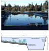
Extended Data Figure 1. Experimental pond used in the study

(a) Photograph of Pond #4 at the experimental pond facility of the University of British Columbia (Vancouver, B.C., Canada), taken in fall of 2008, during the collection of F2 juveniles. (b) Schematic of the pond profile. See Supplementary Discussion 1 for details on pond history prior to this study.

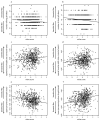
Extended Data Figure 2. Feeding patterns in relation to isotope signatures

Plots show relationships between ingested prey counts from all available F2 hybrids (n = 99) and stable isotope data. (a) Loess-smoothed surface (span = 0.75, 2^nd degree polynomials) of predicted chironomid counts plotted on original isotope axes (δ¹³C, δ¹⁵N). As with all other count data plotted here, counts were transformed as log_e(chironomids+1) and mapped according to the coloured scale. PC1 (black arrow) and PC2 (white) are based on the entire isotope distribution (Fig. 1a). Individuals are plotted as points according to presence (×) or absence (•) of calanoid copepods in their digestive tracts. (b–g) Linear or logistic regression, accordingly, of ingested prey count or presence/absence data (transformed as above) on the different axes through isotope space. Results: (b) chironomid count against δ¹³C, linear regression, slope est. = 0.415, R² = 0.199, F_1,97 = 24.1, P = 3.70×10^-6; (c) chironomid presence against niche score, logistic regression, slope coeff. = 0.504, z = 2.23, P = 0.0255; (d) Collembola presence against diet deviation score, logistic regression, slope coeff. = 1.25, z = 4.26, P = 2.03×10^-5; (e) calanoid count against δ¹⁵N, linear regression, slope est. = 0.492, R² = 0.0608, F_1,97 = 6.28, P = 0.0139; (f) calanoid presence against niche score, logistic regression, slope coeff. = -0.463, z = -1.84, P = 0.0651; (g) calanoid presence against diet deviation score, logistic regression, slope coeff. = -0.958, z = -2.67, P = 0.00766.

Extended Data Figure 3. Linkage map showing QTL for all traits

All G. aculeatus chromosomes are represented by linkage groups (LG) in the complete linkage map for this study (LG and chromosomes use same numbering; LG with no mapped QTL are omitted here). Map distances indicated with scale at left of each LG in centimorgans (cM). Coloured bars (at right) are 1.5-LOD confidence intervals for QTL position (red bars, ‘component traits of niche use’; blue bars, ‘other traits’; Supplementary Table 3 provides LOD scores, map positions of LOD peaks, and effect sizes). The given SNP identifiers (IDs) are only for reference to Supplementary Table 4, which provides published SNP data. For clarity every other ID is omitted for SNP 066–098, even though these markers are present in the map. Markers closest to candidate QTL for genetic model comparisons are highlighted: red text, nearest to candidate QTL for niche score; green boxes, diet deviation score. Numbered traits are x- and y- coordinates of morphometric landmarks (indicated on fish photo): 1, posterior midpoint caudal peduncle; 2, anterior insertion anal fin at first soft ray; 3, posteroventral corner ectocoracoid; 4, posterodorsal corner ectocoracoid; 5, anterior-most corner ectocoracoid; 6, anteroventral corner opercle; 7, posterodorsal corner opercle; 8, dorsal edge opercle-hyomandibular boundary; 9, dorsal-most extent preopercle; 10, posteroventral corner preopercle; 11, anterior-most extent preopercle along ventral silhouette; 12, posteroventral extent maxilla; 13, anterodorsal extent maxilla; 14, suture between nasal and frontal bones along dorsal silhouette; 15, anterior margin orbit; 16, posterior margin orbit; 17, ventral margin orbit (landmarks 15–17 placed in line with vertical or horizontal midpoint of eye); 18, posterior extent supraoccipital along dorsal silhouette; 19, anterior insertion dorsal fin at first soft ray.

Extended Data Figure 4. Shape variation among F2 hybrid groups

Each panel compares mean body shape of individuals in one of three categories of F2 hybrids (‘B’, ‘L’, or ‘A’; shown in dark blue) with the mean shape of all other F2 hybrids (category membership shown in Fig. 1a). Using data for 19 Procrustes-superimposed and unbent landmarks (Extended Data Fig. 3), wireframe diagrams were produced and plotted in MorphoJ ver. 1.04a, based on discriminant function analysis (Supplementary Discussion 7). Shape differences are magnified eightfold for easier visual comparison. Sample sizes: n = 91 (‘B’), n = 92 (‘L’), n = 93 (‘A’), n = 335 (all other F2 hybrids). Supplementary Discussion 7 describes patterns of variation in several specific features of shape, which can be interpreted from these data.

Extended Data Figure 5. Variation of additional traits among F2 hybrid groups

Means (± 1 s.e.m.) of F2 hybrids in groups ‘B’, ‘L’, and ‘A’ (Fig. 1a) are shown for the following traits: (a) number of long gill rakers (ANOVA, F_2,279 = 1.756, P = 0.175); (b) residual epaxial muscle height (F_2,246 = 5.219, P = 0.00603); (c) residual epaxial muscle width (F_2,246 = 4.223, P = 0.0157); (d) neurocranium outlever length (F_2,246 = 13.36, P = 3.10×10^-6); (e) residual buccal cavity length (F_2,246 = 12.26, P = 8.42×10^-6); (f) residual gape (F_2,246 = 7.974, P = 4.41×10^-4). Traits are illustrated in Fig. 2 e–g. The data conformed reasonably well to parametric statistical assumptions, so ANOVA was used to test trait variation among categories.

Extended Data Figure 6. Relationships between F2 hybrid functional morphology and niche score

For key functional morphological traits known to differ between Paxton benthics and limnetics, trait data from all available F2 hybrids are plotted against niche score and fitted with linear regression (raw data for gill raker counts; size-corrected data for other traits): (a) number of long gill rakers (R² = 0.0146; F_1,629 = 9.32; P = 0.00236); (b) number of short gill rakers (R² = 0.0253; F_1,629 = 16.30; P = 6.06×10^-5); (c) residual epaxial muscle height (R² = 0.0125; F_1,552 = 7.00; P = 0.00804); (d) residual epaxial muscle width (R² = 0.0189; F_1,552 = 10.61; P = 0.00119); (e) residual upper jaw protrusion length (R² = 0.0580; F_1,552 = 34.00; P = 9.40 × 10^-9); (f) residual lower jaw-opening inlever length (R² = 0.0660; F_1,615 = 43.43; P = 9.45 × 10^-11). Traits illustrated in Fig. 2 e–g. Directions of benthic–limnetic divergence in Paxton Lake (arrows at left of plots, here and Fig. 2 a–d) are based on previously published studies^,,, combined with validating counts of long and short gill rakers for this study (data not shown).

Figure 1. Niche use and body size

(a) Stable isotopes (δ¹³C, δ¹⁵N) for 625 F2 hybrids, showing contours of loess-smoothed body size (mm). Individuals with extreme loess-predicted size shown as black points (▼ for group ‘B’, ▲ for ‘L’, ■ for ‘A’; each contains 15% of individuals sampled from the pond; ‘L’ restricted to PC1 < 0.045 to preserve group distinctiveness). Other individuals shown as grey circles. Arrows indicate principal components of isotope distribution (PC1, ‘niche score’; PC2, ‘diet deviation score’; origin, red cross). (b–e) Counts of common food items (mean ± 1 s.e.m.) in digestive tracts of ‘B’, ‘L’, and ‘A’ individuals. Kruskal-Wallis tests for differences among groups: larval Chironomidae ( ${\chi }_2^2=13.52$, P = 0.001); S. oregonensis ( ${\chi }_2^2=7.547$, P = 0.023); Collembola ( ${\chi }_2^2=18.67$, P = 8.82×10^-5); Chydorus sp. ( ${\chi }_2^2=0.629$, P = 0.730). (f) Cubic splines of mean body size against ‘niche score’ (predicted values ± 2 s.e.m.) estimated using the 20 largest F2 families (n = 438 individuals), 1,000 bootstrap replicates, and F2 family as a covariate (black, all individuals; orange, individuals with PC2<0).

Figure 2. Trait variation among F2 hybrid groups

Trait means (± 1 s.e.m.) of F2 hybrids in categories ‘B’, ‘L’, and ‘A’ (Fig. 1a): (a) number of short gill rakers (ANOVA, F_2,279 = 5.396, P = 0.005); (b) suction feeding index (F_2,246 = 4.080, P = 0.018); (c) residual lower jaw-opening inlever length (F_2,275 = 20.36, P = 5.65×10^-9); (d) residual upper jaw protrusion length (F_2,246 = 14.94, P = 7.54×10^-7). Trait illustrations: (e) gill rakers, functioning in prey retention^,; (f) five components of suction index^,; (g) two oral jaw traits, which influence efficiency of capturing evasive zooplankton. Arrows indicate directions of benthic–limnetic divergence (vertical axes of b and c inverted to facilitate visual comparisons).

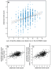
Figure 3. Genetic architecture of niche divergence

(a) Niche scores of F2 hybrids are predicted from the number of benthic alleles summed across eleven unlinked loci (R² = 0.081; F_1,605 = 53.52; P = 8.18×10^-13). Dashed lines are 95% confidence intervals of regression line (solid). (b) Observed niche score compared with that predicted by the additive-only genetic model. (c) Observed niche score compared with that predicted by the full genetic model. Statistics for (b) and (c) are provided in the text.

References

1. Darwin C. The Origin of Species by Means of Natural Selection. John Murray; 1859.
1. Schluter D. The Ecology of Adaptive Radiation. Oxford University Press; 2000.
1. Coyne JA, Orr HA. Speciation. Sinauer Associates, Inc.; 2004.
1. Nosil P. Ecological Speciation. Oxford University Press; 2012.
1. Chase JM, Leibold MA. Ecological Niches: Linking Classical and Contemporary Approaches. The University of Chicago Press; 2003.
Publication types