Single-cell RNA-seq reveals dynamic paracrine control of cellular variation

Abstract

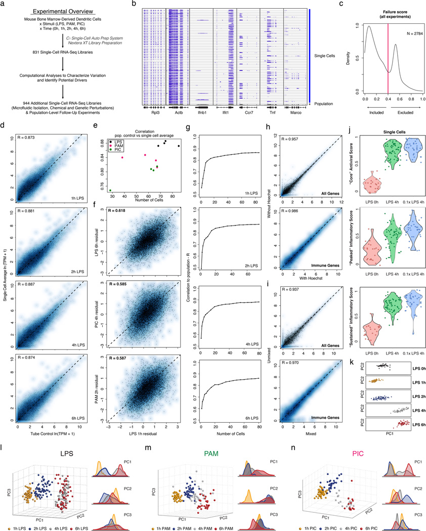
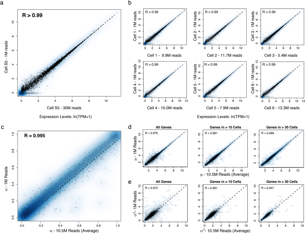
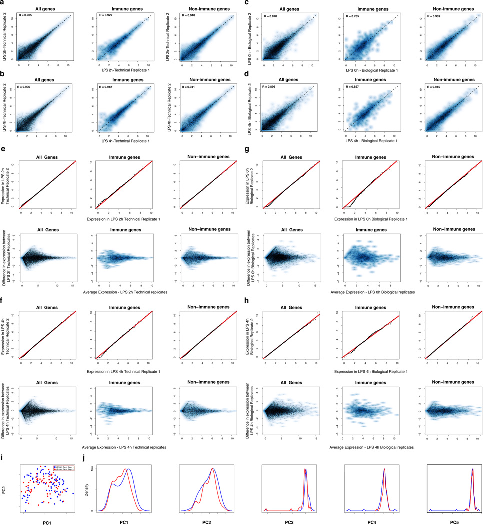
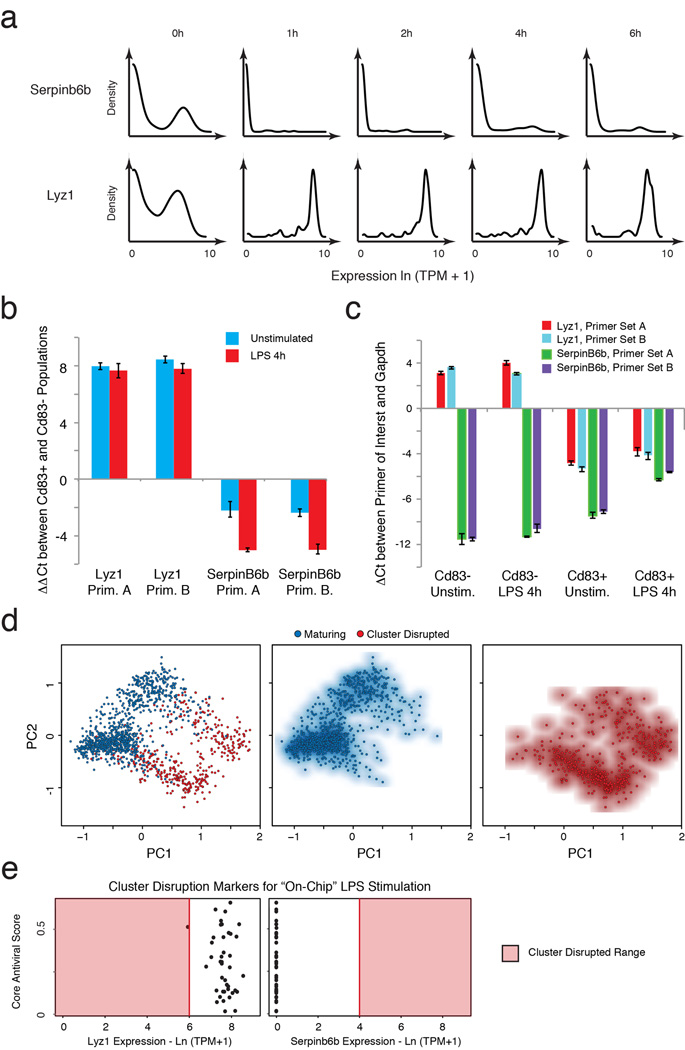
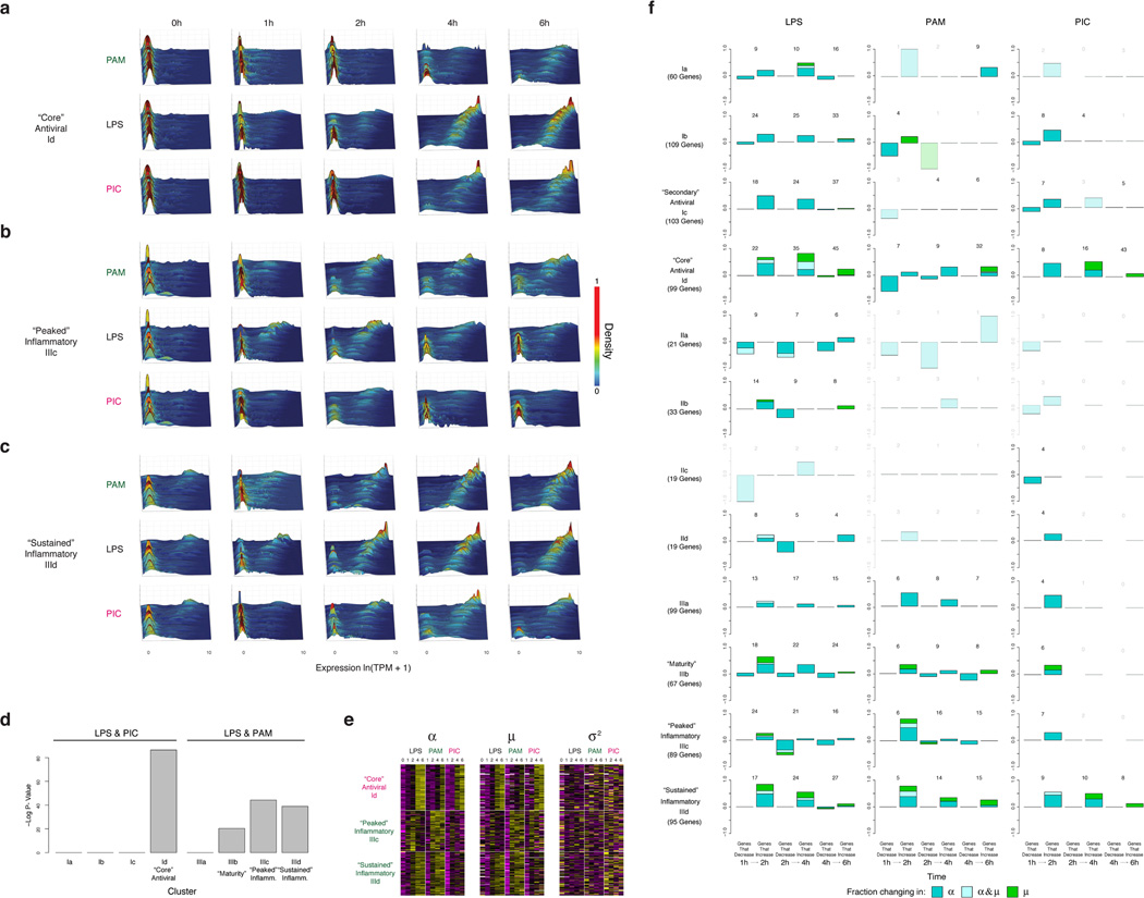
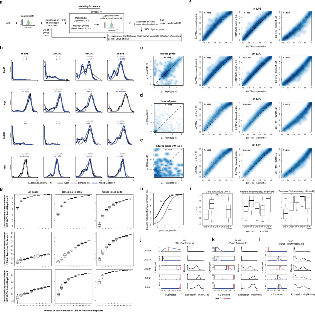
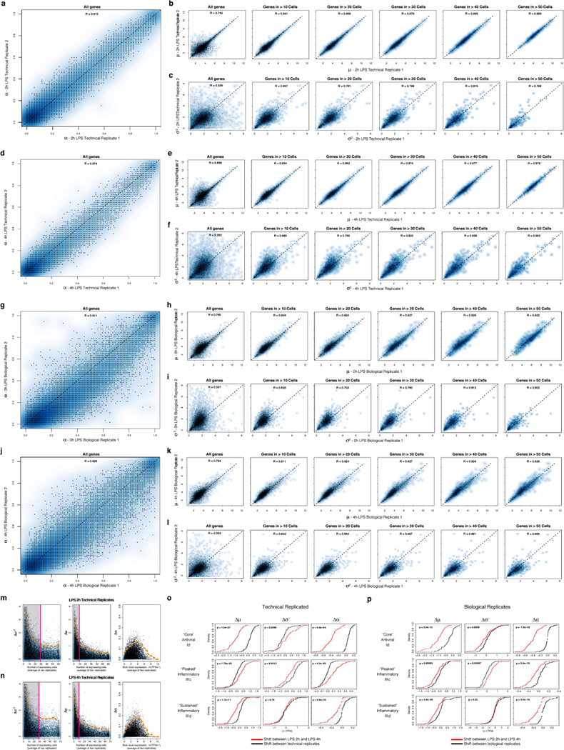
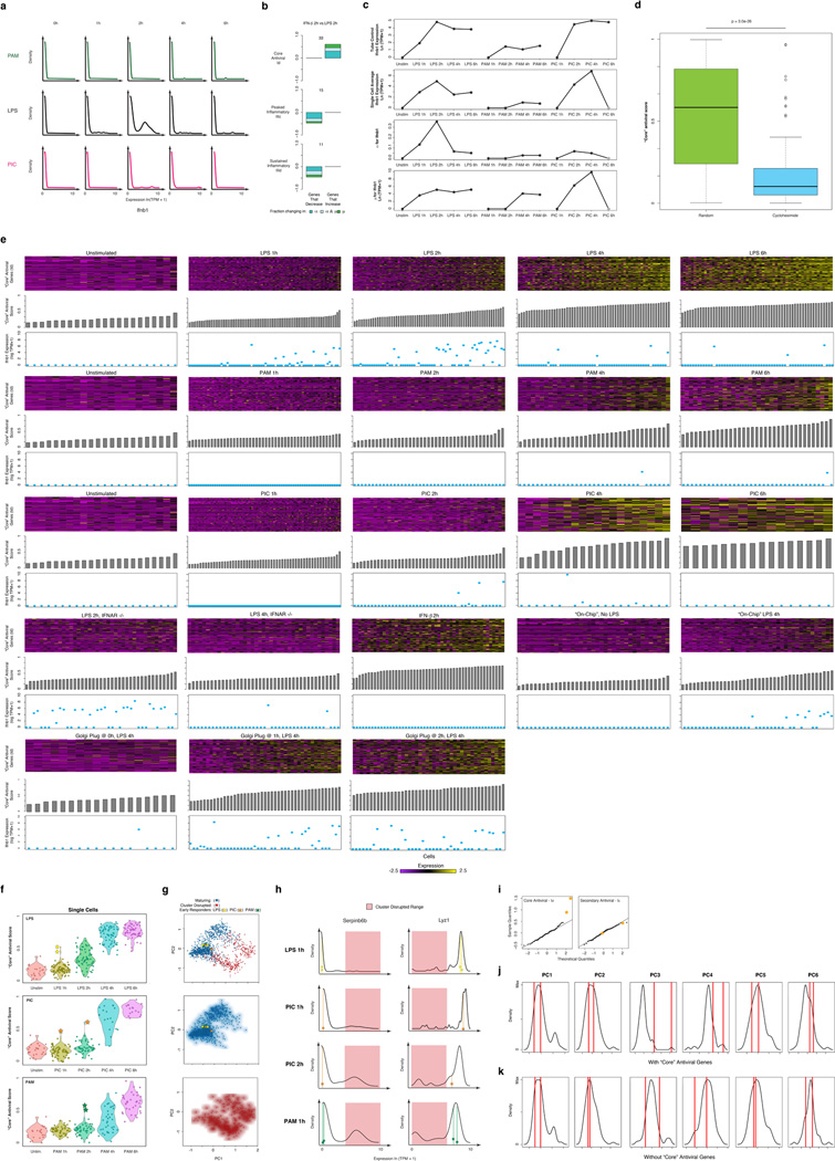
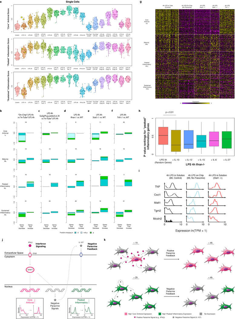
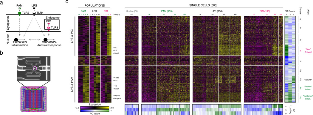
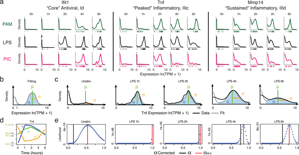
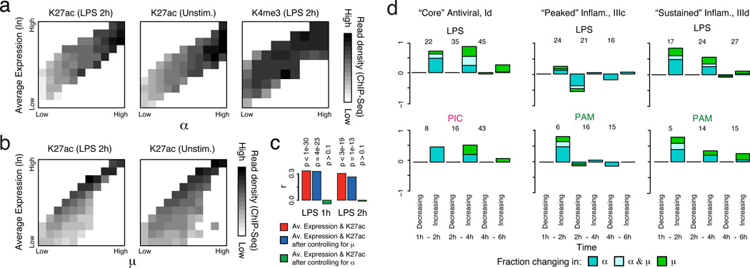
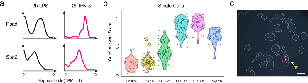
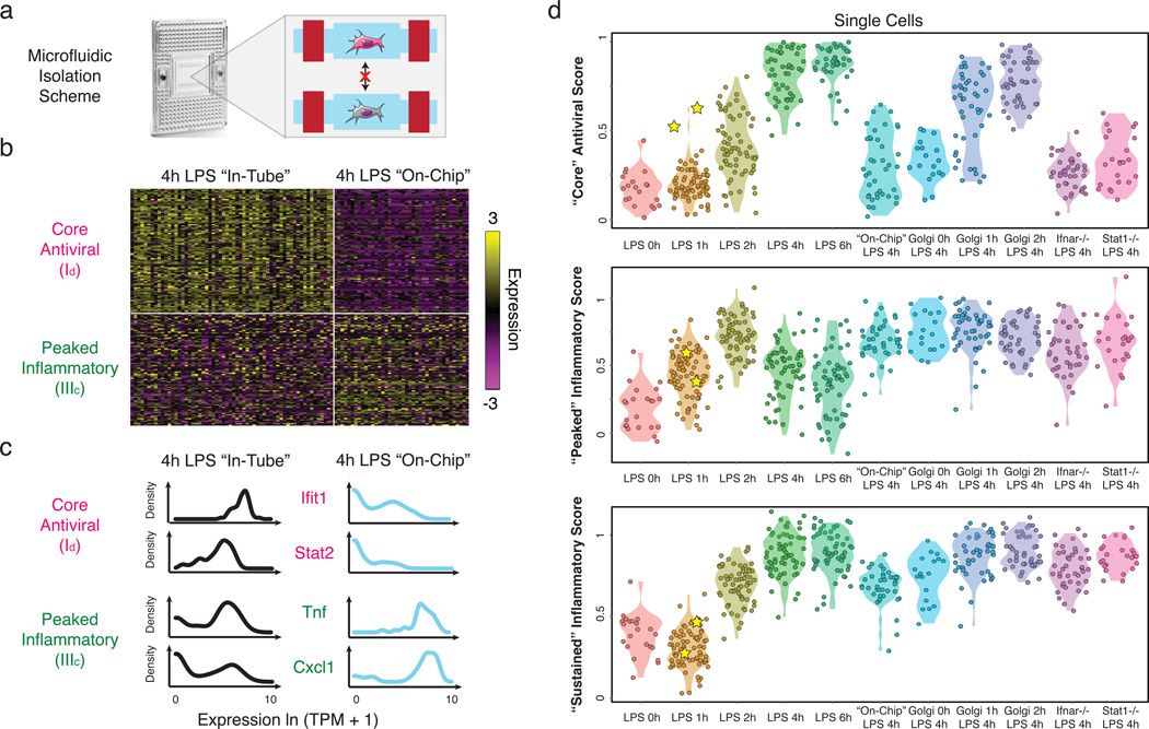
High-throughput single-cell transcriptomics offers an unbiased approach for understanding the extent, basis and function of gene expression variation between seemingly identical cells. Here we sequence single-cell RNA-seq libraries prepared from over 1,700 primary mouse bone-marrow-derived dendritic cells spanning several experimental conditions. We find substantial variation between identically stimulated dendritic cells, in both the fraction of cells detectably expressing a given messenger RNA and the transcript's level within expressing cells. Distinct gene modules are characterized by different temporal heterogeneity profiles. In particular, a 'core' module of antiviral genes is expressed very early by a few 'precocious' cells in response to uniform stimulation with a pathogenic component, but is later activated in all cells. By stimulating cells individually in sealed microfluidic chambers, analysing dendritic cells from knockout mice, and modulating secretion and extracellular signalling, we show that this response is coordinated by interferon-mediated paracrine signalling from these precocious cells. Notably, preventing cell-to-cell communication also substantially reduces variability between cells in the expression of an early-induced 'peaked' inflammatory module, suggesting that paracrine signalling additionally represses part of the inflammatory program. Our study highlights the importance of cell-to-cell communication in controlling cellular heterogeneity and reveals general strategies that multicellular populations can use to establish complex dynamic responses.

Extended Figure 1. Single-cell RNA-Seq of hundreds of DCs

(a) Overview of experimental workflow. (b) Shown are read densities for seven representative genes (two housekeeping genes: Rpl3 and Actb and five immune response genes: Ifnb1, Ifit1, Ccr7, Tnf, Marco) across 60 single cells (blue) and one population control of 10,000 cells (grey) in 4h LPS. (c) Distribution of failure scores for all single cells. Single cells with failure scores above 0.4 were discarded (see SI). (d–g) Comparing expression estimates for the “average” single cell and the bulk population. (d) Scatter plots showing for each gene the relation between the average single-cell expression (Y axis) and bulk population level expression (X axis) for each of four time points following LPS stimulation (1, 2, 4, and 6h, left to right). (e) The Pearson correlation coefficients (Y axis) of each comparison, as in d, for each of the time points and stimuli presented in Fig. 1, as a function of the number of cells captured in the respective experiment (X axis). (f) Scatter plots showing the residual (population-level expression minus the single cell average) in an LPS 1h experiment (X axis) vs. the residual in each of 3 other experiments (Y axis, left to right): LPS 6h, PIC 4h and PAM 2h. (g) The Pearson correlation coefficient (Y axis) between the bulk population level expression and the single-cell expression average when a different number of sub-sampled cells (X axis) is included in the single-cell average. (h,i) Effects of Hoechst dye and periodic mixing on mRNA expression. (h) Comparable expression levels after 4h LPS with the addition of small amounts of Hoechst to aid in cell counting (X axis) and when no dye is used (Y axis), when looking at all genes (left) or only immune response genes (right). (i) Comparable expression levels after 4h LPS with hourly mixing (X axis) or with no mixing (Y axis), when looking at all genes (left) or only immune response elements (right). (j) “Core” antiviral, “peaked” inflammatory, and “sustained” inflammatory module activation scores for a 0.1× LPS stimulation. Shown are Violin plots of the scores (Y axis) for the “core” antiviral (SI, top), “peaked” inflammatory (SI, middle), and “sustained” inflammatory modules (SI, bottom) for each cell in (left to right): LPS 0h, 1× (100 ng/mL) LPS 4h, and 0.1× (10 ng/mL) LPS 4h. (k–n) PCA of stimulated DCs. (k) PCA for the first two PCs for samples from the LPS stimulation time course. From top to bottom: unstimulated/LPS 0h, LPS 1h, LPS 2h, LPS 4h, LPS 6h. (l–n) PCAs (left) and the distributions of scores (right) for each of the first three PCs for samples collected after stimulation with LPS (l), PAM (m), or PIC (n), for 1 (yellow), 2 (blue), 4 (grey) and 6 (red) hours. A single PCA was performed for all cells in all three time courses.

Extended Figure 2. Effects of shallow read depth on expression estimates

(a–b) A million reads per cell are sufficient to estimate expression levels. (a) Scatter plot for a single cell (from Shalek et al., Nature, 2013) showing the relation between expression estimates calculated using 30M reads (X axis) or a sub-sample of 1M reads (Y axis). (b) Scatter plots for six different DCs stimulated for 4h with LPS. Each plot shows the relation between expression estimates calculated using all reads (X axis; number of reads marked on axis label) or a sub-sample of 1M reads (Y axis). In all cases, R > 0.99. Note that although, in principle, no gene should be estimated as present only in a subsample but not the full dataset, this does occur for a very small number of genes (e.g., four genes in Cell 3), representing a nuanced technical error in RNA-Seq estimation. Consider two expressed genes, A and B, from distinct loci, but with a short stretch of sequence identity. At low sequencing depth, if reads only map to the shared region, estimation tools such as RSEM used here can guess erroneously which gene is expressed, such that additional sequencing depth can “flip” the assignment of an uncertain read from gene A to gene B. These cases are extremely rare, and have a negligible effect. (c–e) A million reads per cell are sufficient to estimate µ, σ², and α. Scatter plots showing the relation between α (c), µ (d), and σ² (e) values estimated using 10M reads/cell (on average;×axis) or a sub-sample of 1M reads/cell (y axis) from RNA-Seq libraries prepared from individual DCs stimulated for 4h with LPS. (c) For the vast majority of genes, 1M reads are sufficient to estimate α. For a very small fraction (<0.1%) of weakly expressed genes, estimates of α are improved with increased sequencing depth. For ¼ (d) and σ² (e), estimates are plotted for all genes (left), only genes detected in more than 10 cells (middle), or only those genes detected in more than 30 cells (right).

Extended Figure 3. Technical and biological reproducibility

(a–d) Scatter plots showing the relation between the average single-cell expression estimates in either two technical replicates (LPS 2h (a), LPS 4h (b)) or two biological replicates (Unstimulated/LPS 0h (c), LPS 4h (d)) for all genes (top), immune response genes (middle), or non-immune response genes (bottom). (e–f) QQ plots (top) and MA plots (bottom) showing the similarity in expression estimates for the two LPS 2h technical replicates (e) or the two LPS 4h technical replicates (f). Plots are provided across all genes (left), non-immune response genes (middle), or immune response genes (right). (g–h) QQ plots (top) and MA plots (bottom) showing the similarity in expression estimates for all cells (including cluster-disrupted cells) in the two LPS 0h/unstimulated biological replicates (g) or the two LPS 4h biological replicates (h) across either all genes (left), non-immune response genes (middle), or immune response genes (right). Note, that slight variations in the fraction of cluster-disrupted cells and activation state of one of the two 0h samples results in mild deviations between immune response gene estimates in those biological replicates. (i–j) PCA for the two LPS 4h technical replicates. (i) The first two principal components (PC1 and PC2, X and Y axis, respectively) from a PCA from the two LPS 4h stimulation technical replicates (blue: replicate 1; red: replicate 2). (j) The distributions of scores for cells from each of the two technical replicates on each of the first five PCs (left to right: PC1 to PC5).

Extended Figure 4. Cluster disruption

(a) Single-cell expression distributions for Serpinb6b (a positive marker of cluster disruption) and Lyz1 (a negative marker of cluster disruption) at each time point (marked on top) after stimulation with LPS (all cells included, see SI). Distributions are scaled to have the same maximum height. (b) Difference in mRNA expression as measured by qRT-PCR (with a Gapdh control) between Lyz1 or SerpinB6b in cells pre-sorted before stimulation to express or not express CD83 (CD83⁺ and CD83⁻, respectively), a known cell surface marker of cluster-disrupted cells (see SI). Pre-sorted cells were then either unstimulated (blue) or stimulated (red) with LPS for 4h. (c) Expression of cluster-disruption markers does not change with stimulation. qRT-PCR showing the difference between Gapdh (control) and Lyz1 or SerpinB6b expression in cells pre-sorted on Cd83 either in the presence or absence of simulation with LPS. (d) PCA showing the separation between “maturing” (blue dots) and “cluster-disrupted” (red dots) cells. (e) Expression of cluster disruption markers of cells stimulated with LPS “on chip”. For each cell (black dot) stimulated with LPS “on chip”, shown are the expression levels (X axis) of Serpin6b (cluster disruption cell marker, left) and Lyz1 (normal maturing cell marker, right) vs. its antiviral score (Y axis). With one exception, the cells are clearly “maturing” and not “cluster-disrupted”. Red shading: range of expression in cluster disrupted cells.

Extended Figure 5. Time-dependent behaviors of single cells from different modules and stimuli

(a–c) For each of three key modules – “core” antiviral, I_d (a), “peaked” inflammatory, III_c (b), and “sustained” inflammatory, III_d (c) – shown are wave plots of all of its constituent genes in DCs stimulated with PAM (top), LPS (middle), or PIC (bottom) for 0,1,2,4 and 6h (left to right). X axis: expression level, ln(TPM+1); Y axis: genes; Z axis: single-cell expression density (proportion of cells expressing at that level). Genes are ordered from lowest to highest average expression value at the 4h LPS time point. (d) Contributions of each module to measured variation. Significance of the contribution of modules I_a-I_d and III_a-III_d from Fig. 1 to the variation measured throughout the stimulation time course. Shown is the p-value (Mann-Whitney test) of the tested association between each gene module and the first three PCs, calculated using a statistical resampling method (see SI). Only the “core” antiviral, maturity, and “peaked”/”sustained” inflammatory clusters show statistically significant enrichments with the three PCs. (e) Gene modules show coherent shifts in single-cell expression. Shown are heat maps of scaled α (left), µ (middle), and σ² (right) values (color bar, bottom) in each time course (LPS, PAM, PIC) for the genes in each of the three key modules (rows, modules marked on left). Heat maps are row-normalized across all three stimuli, with separate scalings for each of the three parameters, to highlight temporal dynamics. Genes are clustered as in Fig. 1. (f) Dynamic changes in variation during stimulation in each module. For each module (rows) and stimulus (columns), shown are bar plots of the fraction of genes (Y axis) with a significant change only in α (by a likelihood ratio test, P<0.01, blue), only in µ (Wilcoxon test, P<0.01, green), or in both (each test independently, light blue), at each transition (X axis), in different conditions (marked on top) separated by whether they increase or decrease during that transition. In each module and condition, the proportion is calculated out of the genes in the module that are significantly bimodal (by a likelihood ratio test) in at least timepoint during the LPS response and are expressed in at least 10 cells in both conditions. Their number is marked on top of each bar; conditions with 3 or fewer genes changing are semi-transparent.

Extended Figure 6. Comparison of single-cell RNA-Seq to RNA-FISH

(a–f) Single cell mRNA expression distributions by RNA FISH and single cell RNA-Seq. (a) Representative images of genes analyzed by RNA-FISH at 1 and 4h after LPS stimulation. (b–f) mRNA expression distributions for the housekeeping gene B2m (b), the “peaked” inflammatory gene Cxcl1 (c), the “core” antiviral gene Ifit1 (d), the “sustained” inflammatory gene Il6 (e), and the “peaked” inflammatory gene Tnf (f) measured using either single-cell RNA-Seq (top, black curves) or RNA-FISH (black histograms; no smoothing) in either unstimulated cells (LPS 0h) or cells stimulated with LPS for 1, 2, 4 or 6h. (g–j) Determining the detection limit of single-cell RNA-Seq by comparison to RNA-FISH. For each of 25 genes, we compared single-cell RNA-Seq data (Y axis, this study) to RNA-FISH data (X axis, from Shalek et al., Nature, 2013) based on either their µ values (g,h) or α values (i,j), where for RNA-FISH, “expressing” cells were defined for µ or α calculation at different thresholds (from left to right: at least 1, 4, 5, 10 or 20 copies per cell). (g,i) Data from all 25 genes. (h,j) Data after excluding probes from 5 “cluster-disrupted” gene markers (blue; Ccl22, Ccr7, Irf8, Serpinb6b, Stat4), which are less comparable since there are more cluster-disrupted cells in RNA-FISH experiments, and 2 low quality probes (grey; Pkm2, Fus) that showed very low expression in RNA FISH, but had high expression in both single cell and population-level RNA-seq experiments. SPE (square-root of percent explained, top) represents the square-root of the total variance in the RNA Seq parameter explained by the RNA FISH parameter, under the y=x model.

Extended Figure 7. Fitting gene expression distributions

(a) Flow chart of model fitting. Shown are the key steps in fitting the 3-parameter model. (b) Examples of cases where fitting a multimodal distribution is required. Single-cell expression distributions for (top to bottom) Car13, Rgs1, Ms4a6c, and Klf6 at (left to right) 1, 2, 4, and 6h (marked on top) after stimulation with LPS. Distributions are scaled to have the same maximum height. Data: black lines; Bimodal fits: grey lines; Multimodal fits: blue lines. P values (color-coded) calculated using a goodness-of-fit test (a low P value rejects the fit; see SI). (c–e) Reproducibility of gene-specific fitting of the “undetected” mode, when fitting a mix of two normal distributions to all data points, including those with ln(TPM+1) < 1. (c,d) Scatter plot showing the correlation between µ₁ and µ₂ estimates for the two LPS 4h technical replicates (SI), where µ₁ and µ₂ are the two component means (in decreasing order of magnitude) of the two mixed normal distributions. Estimates for µ₂ correlate poorly between technical replicates, particularly when focusing on genes for which µ₂ is greater than 1 (e), suggesting that the current dataset does not support the use of this additional fit parameter. (f) Robustness of α estimates to small deviations in the threshold. Scatter plots showing the correlation between α estimates determined when using a cutoff of ln(TPM+1) = 1 (X axis) vs. when using a cutoff of ln(TPM+1) = 0.25 (Y axis, left); 0.5 (Y axis, middle) or 2 (Y axis, right) for the LPS time course (top to bottom: 1h, 2h, 4h, and 6h). (g) Saturation curves for estimates of µ, σ₂, and α. Box plots depicting the Pearson correlation coefficient between α (top), µ (middle), or σ₂ (bottom) in two LPS 4h technical replicates, as a function of the number of cells randomly drawn from each replicate (full details in SI). Plots are shown for all genes (left), as well as those detected in more than 10 (middle) or 30 cells, (right) in both replicates (full datasets). (h,i) Correcting for the relationship between mean expression and average detection. (h) The probability of detecting a transcript (Y axis) in a cell as a function of µ (X axis). Black, grey curves are two illustrative cells from the LPS 4h time point. (i) Differences in α_MLE, a stringently-corrected MLE estimate of α (SI), across the LPS time course. Shown are the box plots of α_MLE values (Y axis) for bimodally expressed genes (determined by a likelihood ratio test, SI) at each time point (1, 2, 4, and 6h) following LPS stimulation (X axis), as well as for the “On-chip” 4h LPS stimulation, for each of the “core” antiviral (left), “peaked” inflammatory (middle) and “sustained” inflammatory (right) modules. Stars represent intervals where there is a significant difference in a parameter between two consecutive time points, as determined by a Wilcoxon rank sum test (single star: P<10⁻²; double star: P<10⁻⁵). (j–l) Estimating an upper bound on α using a likelihood test. For each of three transcripts (Ifit1 (j); Rsad2 (k); and Cxcl1 (l)) shown are their expression distributions (red, left) and the matching likelihood function for a stringent upper estimate of α (blue dots, right), when considering a null model where expression is distributed in a lognormal fashion and any deviations are due to technical detection limits (SI). Red vertical line: α_MLE; black vertical line: nominal α. Vertical green bars signify the “nominal” estimation of α, representing the fraction of cells with detected expression of a transcript.

Extended Figure 8. Reproducibility of estimates µ, σ², and α parameters

(a–f) Reproducibility of estimated µ, σ², and α parameters between technical replicates. Scatter plots showing the relation between the estimated α (a), µ (b), and σ² (c) values for the two unstimulated/LPS 0h technical replicates. For µ (b) and σ² (c), estimates are plotted for all genes (leftmost), as well as (left to right) for genes only detected in more than 10, 20, 30, 40, or 50 cells, respectively. (d) – (f) show the same plots for the two LPS 4h technical replicates. (g–h) Reproducibility of estimated µ, σ², and α parameters between biological replicates. Scatter plots showing the relation between the α (g), µ (h), and σ² (i) values estimates for the two LPS 2h biological replicates. For µ (h) and σ² (i), estimates are plotted for all genes (leftmost), as well as (left to right) for genes only detected in more than 10, 20, 30, 40, or 50 cells, respectively. (j) – (l) show the same plots for the two LPS 4h biological replicates. (m,n) Relation between per-gene errors for µ, σ², and α and the number of cells in which the gene’s expression is detected, or its bulk expression level. Scatter plots displaying the differences in the σ² (left), µ (middle), and α (right) estimates for each gene between technical replicates for LPS 2h (m) or LPS 4h (n) (Y axis) as a function of either the number of cells in which the transcript is detected (X axis, for µ and σ²), or the transcript’s bulk expression level (TPM, X axis, for α). Notably, ò (left) estimates saturate (denoted by a magenta line and shaded box) after ~ 30 detectable events, while µ estimates saturate after ~ 10. Dashed orange line: 95% confidence interval. (o,p) Changes in µ, σ², and α between time points are significant as compared to null models from both technical and biological replicates. Shown are the cumulative distribution functions (CDF) for shifts in µ (left), σ² (middle), and α (right) between 2h and 4h (red CDF) for the “core” antiviral (top), “peaked” inflammatory (middle), and “sustained” inflammatory (bottom) modules compared to a null model (black CDF) derived from either technical (o) or biological (p) replicates (SI). In the vast majority of cases, the changes between time points are significant, as assessed by a Kolmogorov-Smirnof (KS) test (P-value of test in the upper left corner of each plot).

Extended Figure 9. Ifnb1 expression, production, and precocious cells

(a–b) Ifnb1 mRNA expression and the effect of IFN-β on variation. (a) Single-cell expression distributions for the Ifnb1 transcript at each time point (top) after stimulation with PAM (top, green), LPS (middle, black), and PIC (bottom, magenta). Distributions are produced with the density function in R with default parameters, and scaled to have the same maximum density. (b) For each of three modules defined in Fig. 1 (core antiviral, top; peaked inflammatory, middle; sustained inflammatory, bottom), shown are bar plots of the fraction of genes (Y axis) with a significant change only in α (by a likelihood ratio test, P < 0.01, blue), only in µ (Wilcoxon test, P < 0.01, green), or in both (each test independently, light blue) between the 2h LPS stimulation and the 2h IFN-β stimulation separated by whether they increase or decrease during that transition. In each module and condition, the proportion is calculated out of the genes in the module that are significantly bimodal (by a likelihood ratio test) in at least time point during the LPS response and are expressed in at least 10 cells in both conditions. Their number is marked on top of each bar. (c–d) Ifnb1 mRNA expression patterns and effect of Cycloheximide. (c) From top to bottom, population average Ifnb1 mRNA expression (top), single-cell average Ifnb1 mRNA expression (second to top), α (second to bottom) and µ (bottom) estimates for Ifnb1 for each stimulation condition in Fig. 1. Grey star at 6h for PIC denotes uncertainty due to the small number of cells captured at that time point. (d) Shown are box plots of the “core” antiviral scores (population level, see SI) after a 4h LPS stimulation either where Cycloheximide was added at the time of stimulation (right, blue), or during a standard 4h LPS control (left, green). “Core” antiviral expression is dramatically decreased with addition of Cycloheximide, suggesting that newly produced protein is needed to initiate the antiviral response. (e) Relationship between “core” antiviral gene expression and Ifnb1 mRNA expression during the LPS, PAM, and PIC stimulation time courses and in follow-up experiments. Shown are the expression of “core” antiviral genes (heat maps: rows – gene; columns – cells) for cells stimulated for 0, 1, 2, 4, or 6 hours (left to right) with LPS (top), PAM (middle), or PIC (bottom). Beneath each heat map, grey bars depict the “core” antiviral score (middle panel, see SI) and blue dots show Ifnb1 mRNA expression for each cell in every heat map. (f–k) Identifying the “precocious” cells. (f) “Core” antiviral scores for cells stimulated with LPS, PIC, and PAM. Shown are violin plots of the core antiviral module scores (SI, Y axis) for each cell from time course experiments (from left: 0,1,2,4, and 6h) of DCs stimulated with LPS (top), PIC (middle) or PAM (bottom). Two “precocious” cells (yellow stars, top panel) have unusually high antiviral scores at 1h LPS (yellow stars, top); similarly “precocious” cells can be seen in PIC at 1 and 2h (orange stars, middle) or in PAM at 2h (turquoise stars, bottom). (g) “Precocious” cells in all three responses are typically maturing cells. PCA showing the separation between “maturing” (blue dots) and “cluster-disrupted” (red dots) cells (top), as well as only maturing (middle) or only cluster-disrupted (bottom) cells (all as also shown in Extended Fig. 4d). The “precocious” cells from each of the responses are marked as stars (colors as in (f)), and all fall well within the “maturing” cells. (h) “Precocious” cells in all three responses express Lyz1 and do not express Serpin6b. Shown are mRNA expression distributions for Serpin6b (cluster disruption cell marker, left) and Lyz1 (normal maturing cell marker, right) in LPS 1h, PIC 1 and 2h, and PAM 1h (top to bottom). The typical range for expression in cluster-disrupted cells is shaded in red. The “precocious” cells from each of the responses are marked as stars (colors as in (f)), and all fall well within the “maturing” cells. (i) Normal quantile plots of the expression of genes from the “core” (cluster I_d, left) and secondary (cluster I_c, right) antiviral clusters at 1h LPS. The two “precocious” cells (yellow stars) express unusually high levels of “core” antiviral genes (left) but not of secondary genes (right). (j,k) The “precocious” cells are only distinguished by the expression of ~100 core antiviral genes. Shown are the distributions of scores for each of the first five PCs (right) for samples collected after stimulation with LPS for 1 hours with (j) or without (k) the inclusion of “core” antiviral genes. “Precocious” cells (vertical red bars), normally distinguished by the 3^rd and 4^th principle components (j), become indistinguishable from all other cells if the ~ 100 “core” antiviral genes are excluded (k) prior to performing the PCA.

Extended Figure 10. Characterizing the “precocious” cells

(a) “Core” antiviral, “peaked” inflammatory, and “sustained” inflammatory module scores during the LPS time course and follow-up experiments. Shown are violin plots of the scores (Y axis) for the “core” antiviral (SI, top), “peaked” inflammatory (SI, middle), and “sustained” inflammatory (SI, bottom) modules for cells in each of the experiments (from left to right): LPS 0h, LPS 1h, LPS 2h, LPS 2h technical replicate 1, LPS 2h technical replicate 2, LPS 4h, LPS 4h technical replicate 1, LPS 4h technical replicate 2, LPS 4h biological replicate, LPS 6h, IFN-β 2h, “On-Chip” unstimulated, “On-Chip” LPS 4h, LPS 4h with GolgiPlug at 0h, LPS 4h with GolgiPlug at 1h, LPS 4h with GolgiPlug at 2h, LPS 4h with Ifnar^−/− DCs, and LPS 4h with Stat1^−/− DCs. Yellow stars: the two “precocious” cells at 1h LPS. (b) Changes in expression and variation during stimulation in the “on-chip”. For genes in the (from top to bottom) “core” antiviral, “maturity”, “peaked” inflammatory, and “sustained” inflammatory modules, shown are bar plots of the fraction of genes (Y axis) with a significant change only in α (by a likelihood ratio test, P<0.01, blue), only in µ (Wilcoxon test, P<0.01, green), or in both (each test independently, light blue) between either the 4h “on-chip” LPS stimulation and the 4h “in-tube” LPS stimulation separated by whether they increase or decrease during that transition. In each module and condition, the proportion is calculated out of the genes in the module that are significantly bimodal (by a likelihood ratio test) in at least timepoint during the LPS response and are expressed in at least 10 cells in both conditions. Their number is marked on top of each bar. (c–f) Bar plots, as in b, for a 4h wild-type LPS stimulation (in tube) and either a 4h “in-tube” LPS stimulation where GolgiPlug was added 2h after LPS (c), a 4h LPS stimulation of Ifnar^−/− DCs (d), a 4h LPS stimulation of STAT1^−/− DCs (e), or a 4h LPS Stimulation of TNFR^−/− DCs (f). (g) Genetic perturbations alter expression and variation in different inflammatory and antiviral modules. Shown is the expression of the genes (rows) in – from top to bottom – the “core” antiviral (I_d), “maturity” (III_b), “peaked” inflammatory (III_c), and “sustained” inflammatory (III_d) modules in single cells (columns) in – from left to right – the “in-tube”, “on-chip”, IFNAR^−/−, STAT1^−/−, and TNFR^−/− conditions. Yellow/purple color scale: scaled expression values (z-scores). (h) Scores of the “peaked” inflammatory module for Ifnar^−/− DCs with recombinant cytokines. Shown are box plots of the “peaked” inflammatory module scores (SI, Y axis) for three population-level replicates of a 4h LPS stimulation of Ifnar^−/− DCs to which a recombinant cytokine (X axis) has been added at 2h after stimulation. Notably, adding IL-10 significantly reduces the “peaked” inflammatory module. (i) Stat1 knockout affects expression and variation of “peaked” inflammatory genes. Shown are expression distributions for five “peaked” inflammatory genes after 4h of LPS stimulation in each of three conditions: “in-tube” stimulation of WT DCs (control; left), “on-chip” stimulation of WT cells (no cell-to-cell signaling; middle), and a stimulation of DCs from Stat1^−/− mice (performed “in-tube”; right). (j,k) Population-level paracrine signaling enhances and coordinates the “core” antiviral response while dampening and desynchronizing the “peaked” inflammatory ones. (j) Gene network model showing how positive IFN-β signaling induces the antiviral response and reduces its heterogeneity, while simultaneously activating a negative paracrine feedback loop, possibly including IL-10, which dampens the “peaked” inflammatory cluster and increases its heterogeneity. (k) Cell population model showing how positive and negative paracrine feedback alter antiviral (magenta) and inflammatory (green) gene expression variability across cells. Grey denotes no expression.

Figure 1. Microfluidic-enabled single-cell RNA-Seq of DCs stimulated with pathogenic components

(a) Schematic of Toll-like receptor (TLR) sensing of PAM by TLR2, LPS by TLR4, and PIC by TLR3 (SI). (b) Microfluidic capture of a single DC (top, cell circled in purple) on a C1 chip (CAD drawing, bottom). (c) Time-course expression profiles for induced genes (rows) in DCs (columns) at 0,1,2,4,&6h post stimulation with PAM (green), LPS (black), and PIC (magenta) within populations (left) and individual cells (right). Far right: gene projection scores onto the first three PCs (columns); bottom: contributions of each cell (columns) to the first three PCs (rows).

Figure 2. Time-dependent behaviours of single cells

(a) Single-cell expression distributions for three genes at each time point after stimulation with PAM (top, green), LPS (middle, black), or PIC (bottom, magenta). Distributions are scaled to have the same maximum height. Individual cells are plotted as bars underneath each distribution. (b) Three parameters describing single-cell expression distributions: µ (green) and σ² (gold), the mean and variance of RNA abundance in detectably expressing cells, respectively, and α (blue), the fraction cells with detectable expression (at ln(TPM+1)>1). (c) Examples of fit (grey) and measured Tnf expression distributions (black). (d) The values of µ, σ², and α (Y axes, left to right) computed for Tnf at each time point (X axis). Units for µ and σ² are ln(TPM+1). (e) Maximum likelihood estimate α(α_MLE). Shown are the likelihood functions (dotted blue line) for Tnf (matching c) used to determine α_MLE (red line; black bar: nominal α; SI).

Figure 3. Dynamic changes in variation during stimulation

(a,b) The relationship between expression and H3K27ac binding depends on α (a), but not on µ (b). Plots show average promoter read density (black high; white low; scale bar, bottom) for H3K27ac in LPS 2h (a,b, left) and unstimulated cells (a, middle; b, right), or H3K4me3 in 2h LPS (a, right) in genes corresponding to each of 10 quantile bins of population expression (Y axis) and each of 10 quantile bins of α (a, X axis) or µ (b, X axis) (SI). (c) Bar plots showing p-values of correlation between average expression levels and K27ac only for immune response genes either as is (red) or when controlling for µ (blue) or α (green). (d) Dynamic changes in α and µ in each module. Bar plots showing for each module the fraction of genes (Y axis) with a significant change only in α (P < 0.01, likelihood ratio test, blue), only in µ (P < 0.01, Wilcoxon test, green), or in both (each test independently, light blue), at each transition (X axis), in different conditions (marked on top). The number of genes over which the proportion is calculated is marked on top of each bar (SI, Extended Fig. 5f).

Figure 4. IFN-β feedback drives heterogeneity in the expression of “core” antiviral targets

(a) Single-cell expression distributions for Rsad (top) and Stat2 (bottom) after stimulating with LPS (left, black) or IFN-β (right, magenta) for 2h. (b) The “core” antiviral score (Y axis; SI, Extended Fig. 9f&10a) for each LPS-stimulated cell at each time point (X axis) and cells simulated for 2h with IFN-β (rightmost). Two “precocious” cells (yellow stars) have unusually high antiviral scores at 1h LPS. (c) RNA-FISH confirms the presence of rare “precocious” responders (arrow; yellow star), positive for both Ifnb1 (magenta) and Ifit1 (cyan). Grey: cell outlines. Scale bar: 25 µm.

Figure 5. Microfluidic blocking of cell-to-cell signaling affects response heterogeneity in “core” antiviral and “peaked” inflammatory modules

(a) Experimental blocking of cell-to-cell communication. Left: C₁ chip; Right: On-chip stimulation, followed by actuation of microfluidic valves (red bars), seals the cells at individual chambers, preventing intercellular signaling. (b) Expression of the genes (rows) in the “core” antiviral (I_d, top rows) and “peaked” inflammatory (III_c, bottom rows) modules in single cells (columns) from the “in-tube” (left) and “on-chip” (right) stimulations. (c) Gene expression distributions for representative genes from the “core” antiviral (top) and “peaked” inflammatory (bottom) modules in the “in-tube” (left, black) or “on-chip” (right, blue) 4h LPS stimulation. (c) Violin plots of, top to bottom, “core” antiviral (SI, top), “peaked” inflammatory (middle), and “sustained” inflammatory (bottom) scores for individual cells from the stimulation conditions listed on the X axis. Yellow stars: the two “precocious” cells from Fig. 4 (Extended Fig. 10a).

References

1. Tay S, et al. Single-cell NF-κB dynamics reveal digital activation and analogue information processing. Nature. 2010;466:267–271. - PMC - PubMed
1. Raj A, Van Oudenaarden A. Single-Molecule Approaches to Stochastic Gene Expression. Annual Review of Biophysics. 2009;38:255–270. - PMC - PubMed
1. Slack MD, Martinez ED, Wu LF, Altschuler SJ. Characterizing heterogeneous cellular responses to perturbations. Proceedings of the National Academy of Sciences. 2008;105:19306–19311. - PMC - PubMed
1. Sharma SV. A chromatin-mediated reversible drug-tolerant state in cancer cell subpopulations. Cell. 2010;141:69–80. - PMC - PubMed
1. Spencer SL, Gaudet S, Albeck JG, Burke JM, Sorger PK. Non-genetic origins of cell-to-cell variability in TRAIL-induced apoptosis. Nature. 2009;459:428–432. - PMC - PubMed
Publication types
Associated data