. 2014 Aug;47(4):369-80.
doi: 10.1111/cpr.12114. Epub 2014 Jun 19.

Oedema-based model for diffuse low-grade gliomas: application to clinical cases under radiotherapy

Affiliations

Oedema-based model for diffuse low-grade gliomas: application to clinical cases under radiotherapy

M Badoual et al. Cell Prolif. 2014 Aug.

Abstract

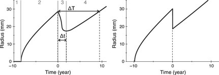
Objectives: Diffuse low-grade gliomas are characterized by slow growth. Despite appropriate treatment, they change inexorably into more aggressive forms, jeopardizing the patient's life. Optimizing treatments, for example with the use of mathematical modelling, could help to prevent tumour regrowth and anaplastic transformation. Here, we present a model of the effect of radiotherapy on such tumours. Our objective is to explain observed delay of tumour regrowth following radiotherapy and to predict its duration.

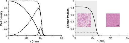
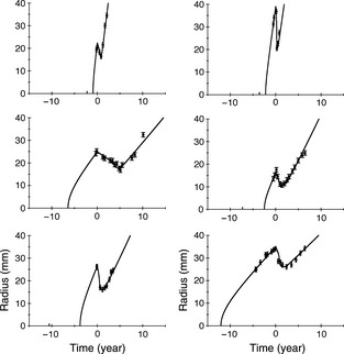
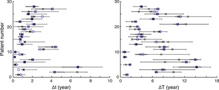
Materials and methods: We have used a migration-proliferation model complemented by an equation describing appearance and draining of oedema. The model has been applied to clinical data of tumour radius over time, for a population of 28 patients.

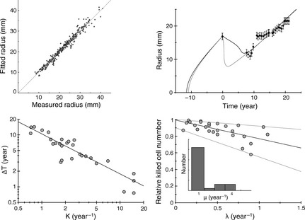
Results: We were able to show that draining of oedema accounts for regrowth delay after radiotherapy and have been able to fit the clinical data in a robust way. The model predicts strong correlation between high proliferation coefficient and low progression-free gain of lifetime, due to radiotherapy among the patients, in agreement with clinical studies. We argue that, with reasonable assumptions, it is possible to predict (precision ~20%) regrowth delay after radiotherapy and the gain of lifetime due to radiotherapy.

Conclusions: Our oedema-based model provides an early estimation of individual duration of tumour response to radiotherapy and thus, opens the door to the possibility of personalized medicine.


Conflict of interest statement

No potential conflicts of interest were disclosed.

Figures

Figure 1
Figure 1
Top: Example of spontaneous velocity of radius expansion of a left temporo‐insular diffuse low‐grade glioma through the evolution of its mean tumour radius on MRI over time. Each point represents an MR examination. Before treatment by radiotherapy (a), the tumour grew spontaneously and continuously. Duration of radiotherapy is indicated by joined arrows. Following radiotherapy, tumour volume measured on follow‐up MRIs decreased for more than 5 years. Then, tumour progression was observed on MRI with a tumour regrowth. Bottom: MRI images corresponding to the times indicated by letters on the radius‐versus‐time curve.
Figure 2
Figure 2
Left: Profiles of cell densities before and after RT. The dashed (respectively solid) black curve corresponds to the cell density profile just before (resp. after) RT. The cell density just after RT is obtained by multiplying the cell density just before RT by a parabola‐shaped function that crosses the horizontal axis at x = R 0. The dotted‐dashed curve is the difference between the solid and the dashed black curves, and represents the cell density that has been killed by RT. The dotted black curve is the density of cells that has been created by proliferation during 6 weeks, between t = −0.12 year and = 0. The parameters are common to all the curves: κ = 7.0 year−1, = 1.75 mm2/year, λ = 0.79 year−1, = 0.60. Right: Example of an oedema fraction curve, at the onset of RT. The parameters are the following: κ = 1.8 year−1, = 0.9 mm2/year, λ = 0.17 year−1, = 0.97 (patient 12). The value of oedema fraction 0.1 (dashed line) is the threshold between the visible part of the tumour on a T2‐weighted MR image (indicated by a grey rectangle) and the invisible part. For the same patient, samples from a biopsy (haematoxylin and eosin staining) inside the MRI‐defined abnormalities are associated with a high fraction of oedema in the tissue [80%, as measured in 14], whereas outside the MRI‐defined abnormalities, the fraction of oedema is lower and reaches zero for normal tissue. The black bar represents 50 μm.
Figure 3
Figure 3
Left: Definition of the regrowth delay Δ t and of the gain of lifetime due to RT Δ T and of the four phases that compose the radius‐versus‐time curve. Right: A radius‐versus‐time curve, with the migration–proliferation model without oedema (the radius of the tumour visible on MRI is calculated from the cell density). The threshold of visibility on the cell density is set to 0.02 37. The parameters are the following: κ = 1.0 year−1, D = 1 mm2/year, λ = 0.5 year−1, = 0.63.
Figure 4
Figure 4
Top: Influence of the parameters on the radius‐versus‐time curve. Thick solid black curve: κ = 1.0 year−1, D = 1 mm2/year, μ = 1.0 year−1, λ = 0.5 year−1, = 0.90; thick solid grey curve: same parameters as for the thick solid black curve, except κ = 2.0 year−1; dashed grey curve: same parameters as for the thick solid black curve, except = 0.74; thin solid black curve: same parameters as for the thick solid black curve, except λ = 0.1 year−1; dashed black curve: same parameters as for the thick solid black curve, except μ = 0.65 year−1. Bottom: Influence of the parameters of the model on ΔT (left) and on Δt (right). The variation of ΔT and Δt (year) obtained by simulation are plotted against the parameters of the model: white triangles for the oedema production coefficient μ (year−1), grey squares for the diffusion coefficient D (mm2/year), crosses for the proliferation coefficient κ (year−1), white circles for the fraction of glioma cells killed by RT x, black circles for the draining coefficient λ (year−1). The solid lines are the best fits (with μ = 1 year−1): ΔT = 7.7/D 0.37; ΔT = 8.1/κ0.72; ΔT = 2.6x/(1.05 − x)0.68; ΔT = 7.8/(1.134 − λ)−0.05.
Figure 5
Figure 5
Superimposition of the tumour radius from patients (black dots) and the fit obtained with our model (solid line), versus time, for six patients. Top left: patient 1, κ = 15 year−1, = 4.8 mm2/year−1, μ =2.8 year−1, λ = 0.6 year−1, = 0.99; top right: patient 5, κ = 15 year−1, D = 3.75 mm2/year−1, μ = 3.2 year−1, λ = 1.8 year−1, = 0.95; middle left: patient 12, κ = 1.8 year−1, =  0.89 mm2/year−1, λ = 0.17 year−1, = 0.97; middle right: patient 19, κ = 4.2 year−1, = 1.06 mm2/year−1, μ = 0.4 year−1, λ = 0.2 year−1; = 0.97; bottom left: patient 16, κ = 3.2 year−1, = 1.6 mm2/year−1, λ = 0.6 year−1, = 0.92; bottom right: patient 25, κ = 1.5 year−1, = 0.78 mm2/year−1, λ = 0.5 year−1, = 0.82.
Figure 6
Figure 6
Top left: The tumour radii obtained by simulations for the 28 patients are plotted against the experimental radii measured on clinical pictures. The coefficient of determination of the linear regression is R 2 = 0.96. Top right: Example of the series radius‐versus‐time for a patient, that can be fitted with different set of parameters, with a comparable mean square difference between the simulated and the experimental data, χ2. In this case, the uncertainty on the measure of Δt is large (see Fig. 7 left, patient 4). Bottom left: The gain of lifetime due to RT ΔT is plotted against κ, in a log‐log scale. The equation of the linear regression is y = 10.4/x 0.76. Bottom right, inset: histogram of distribution of the oedema production μ obtained when fitting all the patients. The relative cell number killed by RT is plotted against the draining coefficient λ, with the best linear regression (y = −0.22x + 0.99) and the two linear curves that comprise all the data points (y = −0.08x + 1 and y = −0.35x + 0.9).
Figure 7
Figure 7
The different Δ t (left) and Δ T (right). The measured values with the associated error bars (thick grey lines), the simulated values in the general case with the four free parameters (white circles), the simulated values with μ fixed to 1 year−1and κ fixed to its minimum value compatible with the constraints (crosses), the simulated values with μ fixed to 1 year−1, κ fixed to its minimum value compatible with the constraints and x calculated from the linear relation with the draining coefficient (squares) (in this case, the error bars correspond to the different linear regressions, see Fig. 5 bottom right).

Similar articles

Cited by

References

    1. Louis DN, Ohgaki H, Wiestler OD, Cavenee WK, Burger PC, Jouvet A et al (2007) The 2007 WHO classification of tumours of the central nervous system. Acta Neuropathol. 114, 97–109. - PMC - PubMed
    1. Pallud J, Mandonnet E (2011) Quantitative approach of the natural course of diffuse low‐grade gliomas In: Hayat MA, ed. Tumors of the Central Nervous System, Vol. 2, pp. 163–172. Netherlands: Springer.
    1. Price SJ (2010) Advances in imaging low‐grade gliomas. Adv. Tech. Stand. Neurosurg. 35, 1–34. - PubMed
    1. Pallud J, Fontaine D, Duffau H, Mandonnet E, Sanai N, Taillandier L et al (2010) Natural history of incidental WHO grade II gliomas. Ann. Neurol. 68, 727–733. - PubMed
    1. Daumas‐Duport C, Meder JF, Monsaingeon V, Missir O, Aubin ML, Szikla G (1983) Cerebral gliomas: malignancy, limits and spatial configuration‐comparative data from serial stereotaxic biopsies and computed tomography (a preliminary study based on 50 cases). J. Neuroradiol. 10, 51–80. - PubMed