Review
doi: 10.1249/JES.0000000000000015.
Dynamic ultrasound imaging applications to quantify musculoskeletal function
Affiliations
- PMID: 24949846
- PMCID: PMC4066199
- DOI: 10.1249/JES.0000000000000015
Item in Clipboard
Review
Dynamic ultrasound imaging applications to quantify musculoskeletal function
Exerc Sport Sci Rev.
2014 Jul.
Erratum in
- Exerc Sport Sci Rev. 2014 Oct;42(4):193
Abstract
Advances in imaging methods have led to new capability to study muscle and tendon motion in vivo. Direct measurements of muscle and tendon kinematics using imaging may lead to improved understanding of musculoskeletal function. This review presents quantitative ultrasound methods for muscle dynamics that can be used to assess in vivo musculoskeletal function when integrated with other conventional biomechanical measurements.
Figures
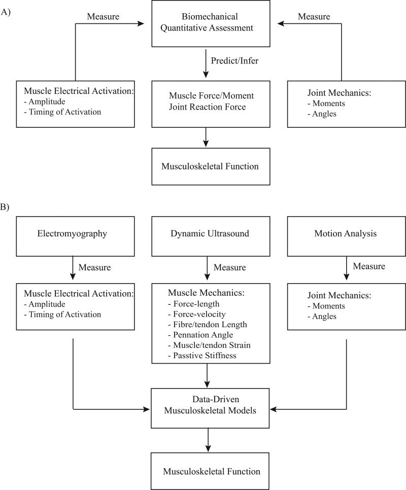
A) Traditional, and B) integrative biomechanical framework for assessment and quantification of dynamic musculoskeletal function.
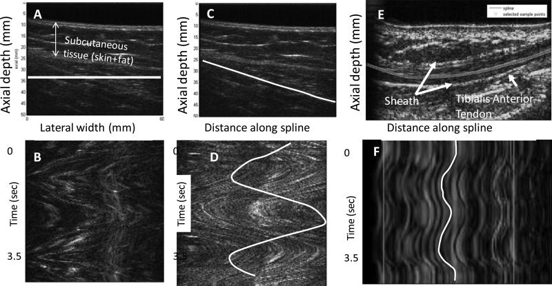
A) Gray-scale B-mode image of rectus femoris muscle during repetitive flexion and extension. (B) M-mode image reconstructed by resampling pixels along the horizontal line indicated in white. The M-mode image shows the pattern of muscle motion back and forth over the course of the knee flexion and extension experiment. (C) A manually initialized curve indicating the approximate orientation of the fascicles. (D) M-mode image reconstructed by resampling pixels along the curved line in (C). The sinusoidal pattern of the muscle contraction and relaxation during knee flexion and extension is clearly visualized. A comparison of the patterns in (C) and (D) demonstrates that to obtain the true pattern of motion, the curve should be aligned with the fascicle direction. (E) B-mode image of the tibialis anterior tendon with a spline curve indicating the location of the tendon. (F) Resampled M-mode image of tibialis anterior tendon generated by sampling pixels along the curve through time. Two cycles of dorsiflexion and relaxation are shown. (Reproduced with permission from IEEE (17)).
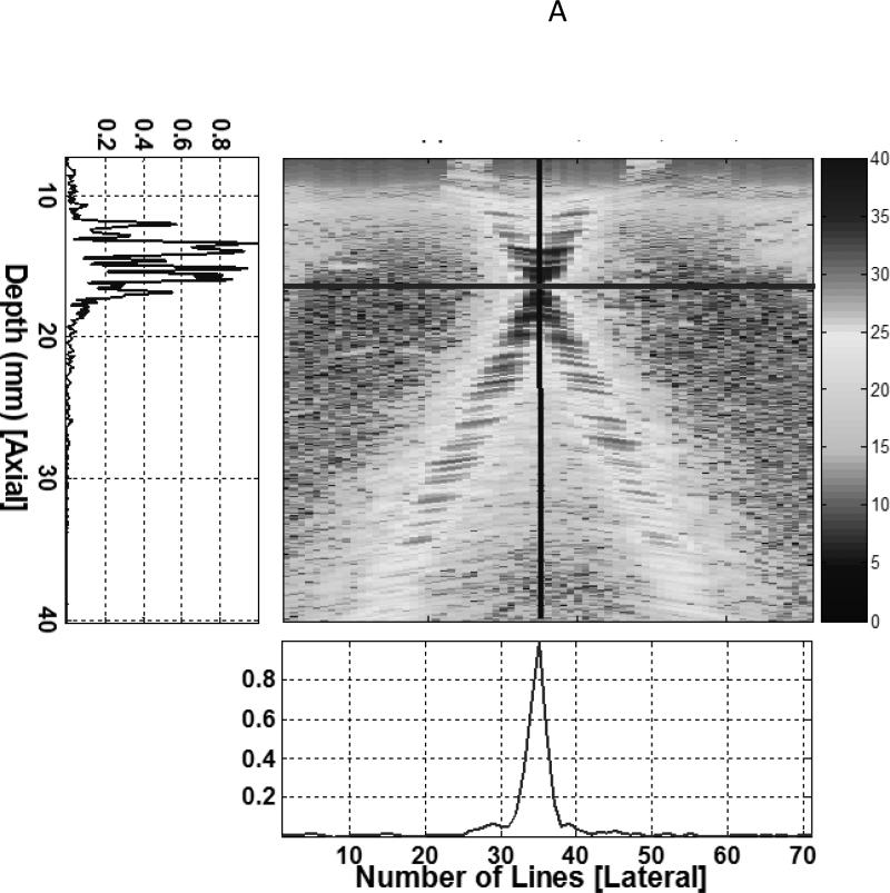
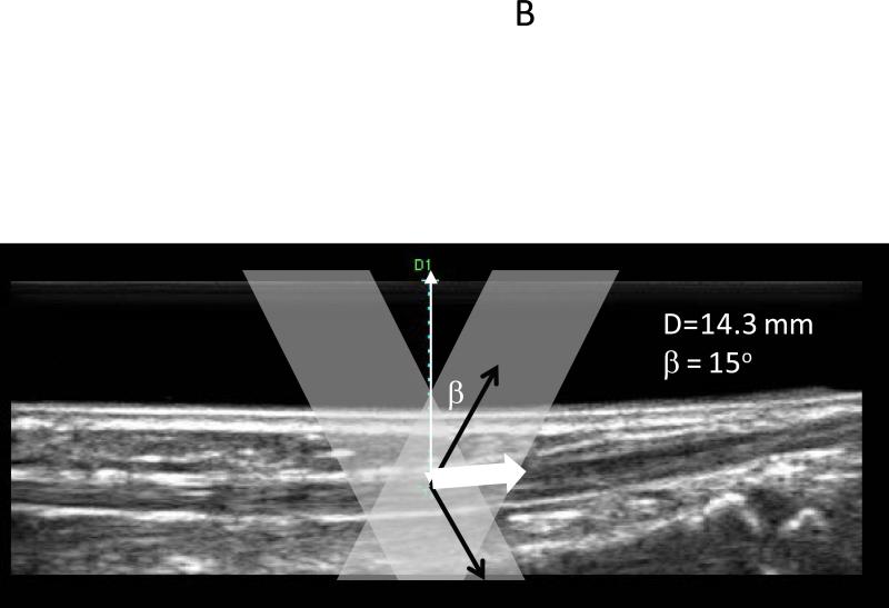
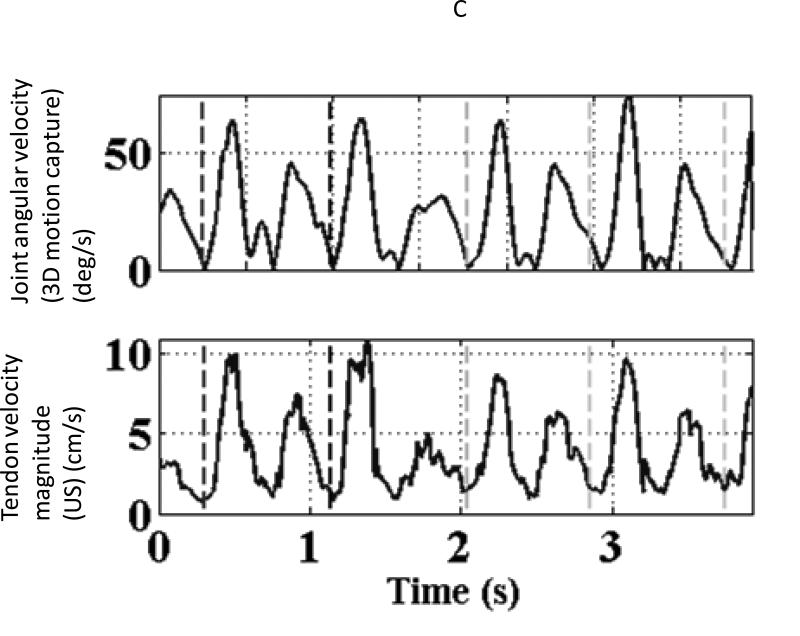
(A) The beam profiles for a vector Doppler imaging visualized using a beam profile phantom. The overlap region between the beams can be adjusted to different depths electronically by changing the separation between the two apertures. (B) B-mode image showing the anterior tibialis tendon visualized at a depth of 14 mm. The overlay denotes a schematic of the two-ultrasound beams used for vector Doppler imaging. The beams were steered at 15° with respect to the normal and velocity estimation was done using 2D Fourier transform. The individual velocity estimates (black arrows) along each beam can be combined geometrically to yield the resultant velocity vector (solid white arrow) (C) Joint angular velocities and corresponding velocity waveforms of the tibialis anterior tendon measured using vector Doppler during four cycles of dorsiflexion and relaxation. The peak magnitude of the velocity vector of the tendon is plotted, and this velocity magnitude was obtained from two separately measured components: axial (perpendicular to the ultrasound transducer) and lateral (parallel to the ultrasound transducer). The separate components are not shown. (Reproduced with permission from IEEE (14)).
(A) The beam profiles for a vector Doppler imaging visualized using a beam profile phantom. The overlap region between the beams can be adjusted to different depths electronically by changing the separation between the two apertures. (B) B-mode image showing the anterior tibialis tendon visualized at a depth of 14 mm. The overlay denotes a schematic of the two-ultrasound beams used for vector Doppler imaging. The beams were steered at 15° with respect to the normal and velocity estimation was done using 2D Fourier transform. The individual velocity estimates (black arrows) along each beam can be combined geometrically to yield the resultant velocity vector (solid white arrow) (C) Joint angular velocities and corresponding velocity waveforms of the tibialis anterior tendon measured using vector Doppler during four cycles of dorsiflexion and relaxation. The peak magnitude of the velocity vector of the tendon is plotted, and this velocity magnitude was obtained from two separately measured components: axial (perpendicular to the ultrasound transducer) and lateral (parallel to the ultrasound transducer). The separate components are not shown. (Reproduced with permission from IEEE (14)).
(A) The beam profiles for a vector Doppler imaging visualized using a beam profile phantom. The overlap region between the beams can be adjusted to different depths electronically by changing the separation between the two apertures. (B) B-mode image showing the anterior tibialis tendon visualized at a depth of 14 mm. The overlay denotes a schematic of the two-ultrasound beams used for vector Doppler imaging. The beams were steered at 15° with respect to the normal and velocity estimation was done using 2D Fourier transform. The individual velocity estimates (black arrows) along each beam can be combined geometrically to yield the resultant velocity vector (solid white arrow) (C) Joint angular velocities and corresponding velocity waveforms of the tibialis anterior tendon measured using vector Doppler during four cycles of dorsiflexion and relaxation. The peak magnitude of the velocity vector of the tendon is plotted, and this velocity magnitude was obtained from two separately measured components: axial (perpendicular to the ultrasound transducer) and lateral (parallel to the ultrasound transducer). The separate components are not shown. (Reproduced with permission from IEEE (14)).
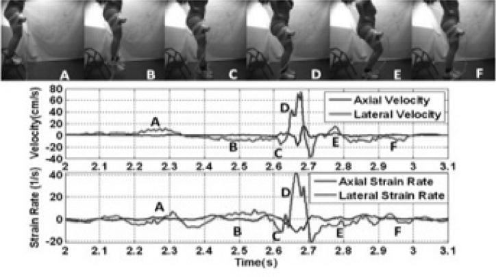
The experimental setup for measuring the rectus femoris muscle velocities and strain rate during a drop-landing task, and representative values of the axial and lateral velocities, and strain rate during the drop-landing task. The top panel shows representative frames from a high speed motion capture showing different phases of the drop landing. The middle panel shows the measured axial (perpendicular to the transducer) and lateral (parallel to the ultrasound transducer) velocity waveforms of the rectus femoris muscle, measured using vector Doppler. The bottom panel shows the corresponding strain rates (spatial derivative of velocity). The different phases of the drop landing task are indicated with the letters A-F corresponding to the frames from the high speed video. (Reproduced with permission from IEEE (15)).
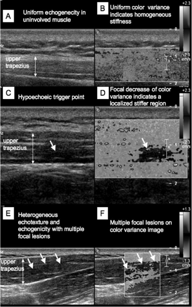
Simultaneous 2D grayscale and color variance imaging. (A and B) Normal upper trapezius muscle. The normal muscle appears isoechoic and has uniform color variance (C and D) Muscle with a palpable MTrP. A hypoechoic region and a well-defined focal decrease of color variance indicating a localized stiffer region are visible. (E and F) Muscle with palpable MTrPs. Multiple hypoechoic regions and multiple focal nodules are visible. (Reproduced with permission from APMR (41)).
References
-
- Asakawa DS, Nayak KS, Blemker SS, et al. Real-time imaging of skeletal muscle velocity. Journal of magnetic resonance imaging : JMRI. 2003;18(6):734–9. - PubMed
Publication types
MeSH terms
Grants and funding
LinkOut - more resources
Full Text Sources
Other Literature Sources