Image reconstruction: an overview for clinicians

Abstract

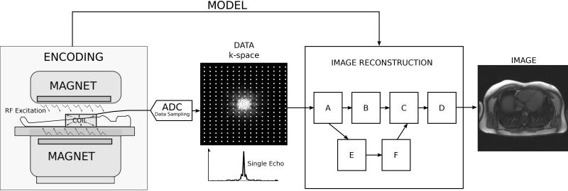
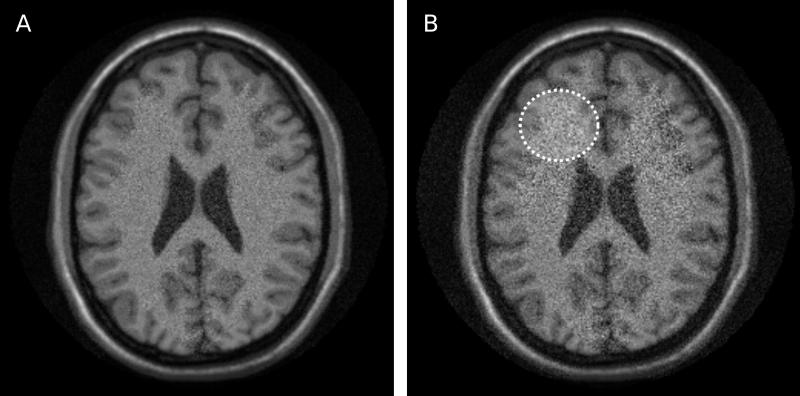
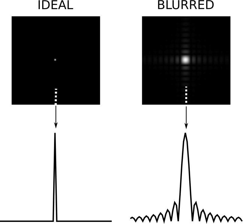
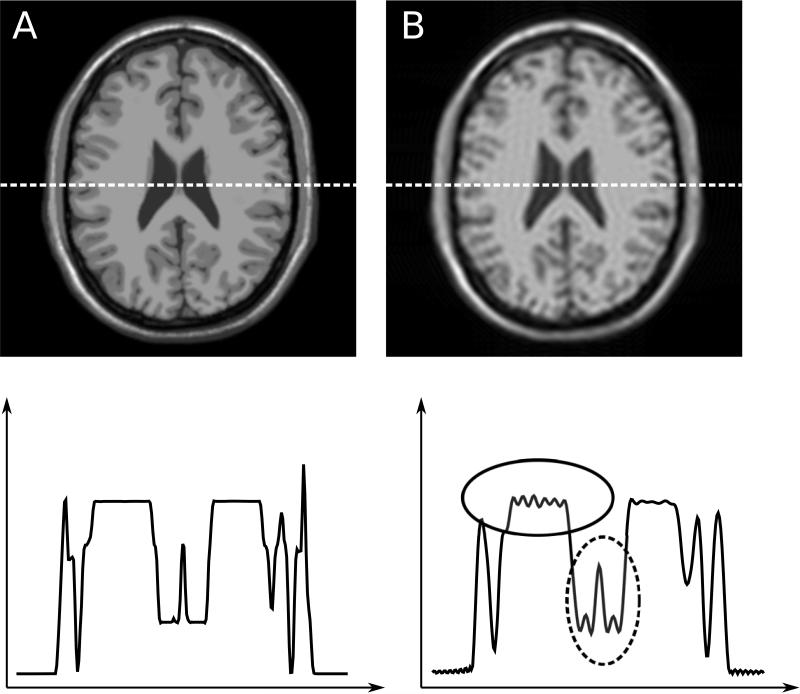
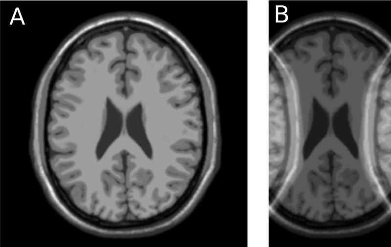
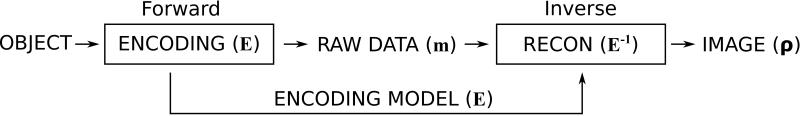
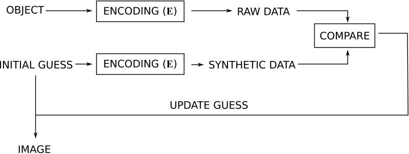
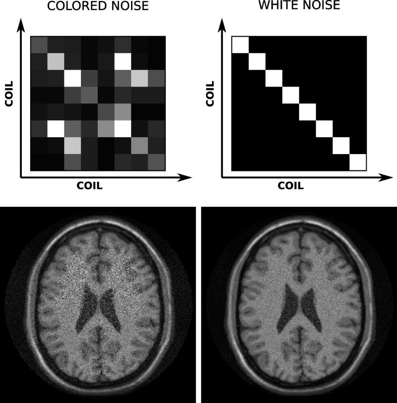
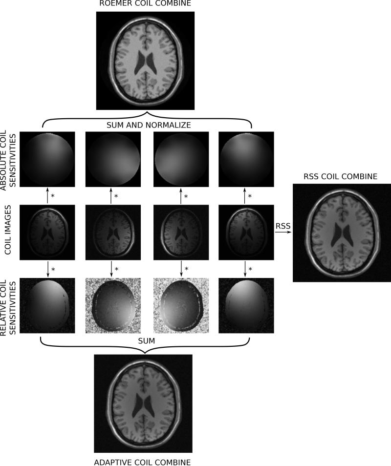
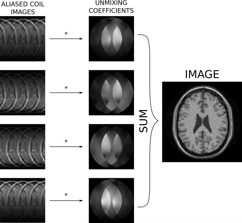
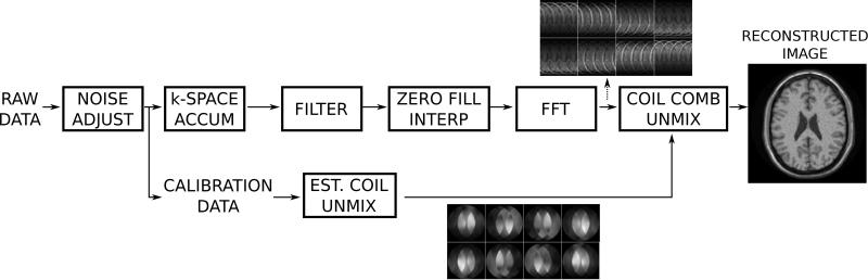
Image reconstruction plays a critical role in the clinical use of magnetic resonance imaging (MRI). The MRI raw data is not acquired in image space and the role of the image reconstruction process is to transform the acquired raw data into images that can be interpreted clinically. This process involves multiple signal processing steps that each have an impact on the image quality. This review explains the basic terminology used for describing and quantifying image quality in terms of signal-to-noise ratio and point spread function. In this context, several commonly used image reconstruction components are discussed. The image reconstruction components covered include noise prewhitening for phased array data acquisition, interpolation needed to reconstruct square pixels, raw data filtering for reducing Gibbs ringing artifacts, Fourier transforms connecting the raw data with image space, and phased array coil combination. The treatment of phased array coils includes a general explanation of parallel imaging as a coil combination technique. The review is aimed at readers with no signal processing experience and should enable them to understand what role basic image reconstruction steps play in the formation of clinical images and how the resulting image quality is described.

Keywords: Gibbs ringing; image reconstruction; noise correlation; point spread function; raw data filtering; signal to noise ratio.

Figure 1

The role of the reconstruction process in the MRI measurement. The MRI hardware with radiofrequency transmit/receive system and spatial encoding gradients serves as the image encoding device. The actual measurement produces encoded imaging data (k-space), which is transformed by the image reconstruction process into images. The task of the image reconstruction process is to use information (a model) about the performed encoding steps to transform the data into images. The reconstruction process consists of multiple signal processing steps that are frequently depicted as steps in a reconstruction pipeline; here the steps are enumerated A-F.

Figure 2

Illustration of reconstructions with different signal to noise ratio (SNR). Image A has higher overall SNR than image B. Furthermore, image B shows varying SNR levels in different image regions. The dotted circle illustrates an area with elevated noise and thus lower SNR.

Figure 3

Illustration of point spread functions. The two images on the top row show reconstruction results of simulated data from a numerical phantom with a single point source of signal. The image on the left shows an idealized scenario where all frequency components of the object are captured and the point source results in a single bright pixel. The image on the right was obtained with a simulated acquisition, which had lower spatial resolution. The lower row shows a plot of a single column of the point spread function for the column indicated by the arrow and dotted line.

Figure 4

Illustration of point spread function effect on simulated neuro images. The image on the left (A) has a simulated point spread function similar to A in Fig. 3. The image on the right (B) is affected by point spread function B of Fig 3. The plots on the bottom row show signal intensity plots corresponding to the row of pixels indicated by the dotted lines in the images. The image on the right appears blurred and exhibits Gibbs ringing. Note how the narrow structure in the central part is blurred out in image B as indicated by the dashed circle. Also note the clear Gibbs ringing artifacts indicated by the solid circle.

Figure 5

Illustration of aliasing or fold over artifact. The image on the right (B) was acquired with half the field of view of the image on the left (A). Signal outside the field of view is erroneously assigned to pixels within the field of view.

Figure 6

Basic workflow for direct reconstruction. The object is subjected to an encoding process and a description of this encoding is captured in a model, which is forwarded to the reconstruction process. The reconstruction process inverts the forward model directly and applies the inverse model on the data to obtain the image result.

Figure 7

Basic workflow for iterative reconstruction. Compared to the direct reconstruction in Fig. 6, the inverse model is never explicitly applied to the data. Instead, an initial guess of what the image could look like is made. This guess could be that all pixels are zero. The guess is subjected to the forward model and synthetic raw data is generated. This synthetic raw data is then compared to the actual acquired data and the difference (residual) is used to update the guess and the process is repeated until the difference between acquired and synthetic data is sufficiently small.

Figure 8

Example of noise pre-whitening in a simulated neuro case. On the top left is a graphical rendering of the coil noise covariance matrix in the case where the noise levels are different in each channel and there is also some significant correlation between certain coil elements as indicated by the off diagonal elements. A direct reconstruction with this noise distribution yields the image on the lower left. The right hand side of the figure shows the results after noise pre-whitening. Now the effective noise covariance matrix is the identity matrix and the image shows marked improvement in the SNR.

Figure 9

An in vivo example of the effects of noise pre-whitening. On the left (A) is seen a direct reconstruction without pre-whitening in a case where a single coil element pre-amplifier was defective and added noise to the measurement. The images were non-diagnostic without the pre-whitening. After pre-whitening, the defective coil element was attenuated and the images were diagnostic.

Figure 10

Illustration of effects of raw data filtering on simulated neuro images. The top row is equivalent to the image in Fig. 4B, which was affected by the point spread function in Fig. 3B. There is considerable Gibbs ringing artifact highlighted by the dotted circle. The three bottom rows represent three different raw filters. The raw filters are all Gaussian shapes where the edge of the window has been set at 1.0, 1.5, and 2.0 times σ. Notice how the filters are progressively better at attenuating the Gibbs ringing albeit at the expense of a broadening of the point spread function.

Figure 11

In vivo cardiac example of raw data filtering. The image on the left is reconstructed with no raw data filtering and there is evidence of Gibbs ringing artifacts in the interventricular septum as highlighted by the plot in the lower part of the figure. After filtering with a Gaussian filter with the edge of k-space set at 1.5* σ, the Gibbs ringing artifact is reduced. In the plot on the bottom right, the unfiltered profile through the interventricular septum is plotted with a dotted line and the filtered profile with a solid line.

Figure 12

Illustration of anisotropic resolution in a simulated neuro dataset. A) Full resolution image acquired with 256x256 samples in k-space and reconstructed on a 256x256 matrix. B) 256x64 (25% phase resolution) acquisition reconstructed on a 256x64 matrix. C) 256x64 acquisition reconstructed on a 256x256 matrix. A Gaussian raw data filter with 1.5*σ width was used in the phase encoding direction. The plot on the bottom depicts line plots in the horizontal direction; image A is represented with a solid line and image C with a dotted line. Notice the reduced resolution (blurring) in the phase encoding direction of image C.

Figure 13

Illustration of commonly used coil combination schemes. Four coil images are show in the central row of the figure. To the right of the coil image is an illustration of a simple but commonly used coil combination method; the root-sum-squares (RSS) coil combination. Above and below the coil images are two different sets of coil sensitivity maps. On the top, absolute coil sensitivities have been used to generate a B1-weighted coil combination with uniform intensity. On the bottom relative coil sensitivities have been used to generate an adaptively combined image.

Figure 14

Illustration of coil combination in the case of parallel imaging with acceleration factor 4 in simulated neuro images. When parallel imaging is employed, a set of coil combination coefficients (unmixing coefficients) are estimated such that these coefficients a) remove the aliasing signal, and b) optimize the signal to noise.

Figure 15

Illustration of a typical reconstruction pipeline for a Cartesian parallel imaging acquisition. The first step in the reconstruction is noise pre-whitening (noise adjust), which removes noise correlation in the data. The data pipeline then splits into two, one for the main image reconstruction and one for the processing of calibration data to form parallel imaging unmixing coefficients. The main processing pipeline performs raw data filtering, zero filling in k-space to ensure square pixels (image interpolation), Fourier transform, and finally coil combination using the parallel imaging unmixing coefficients. This final step turns the aliased channel images into a single combined image.

References

1. Hinshaw WS, Lent AH. An introduction to NMR imaging: From the Bloch equation to the imaging equation. Proc. IEEE. 1983;71:338–350.
1. Ljunggren S. A simple graphical representation of fourier-based imaging methods. J. Magn. Reson. 1983;54:338–343.
1. Twieg DB. The k-trajectory formulation of the NMR imaging process with applications in analysis and synthesis of imaging methods. Med. Phys. 1983;10:610–21. - PubMed
1. Hennig J. Review article K-space sampling strategies. Eur. Radiol. 1999;1031:1020–1031. - PubMed
1. Pauly JM, Nishimura DG, Macovski A. Introduction to: A k-space analysis of small-tip-angle excitation. J. Magn. Reson. 2011;213:558–559. - PubMed
Publication types