

Determining absolute protein numbers by quantitative fluorescence microscopy
- PMID: 24974037
- PMCID: PMC4221264
- DOI: 10.1016/B978-0-12-420138-5.00019-7
Determining absolute protein numbers by quantitative fluorescence microscopy
Abstract
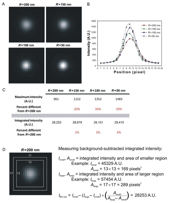
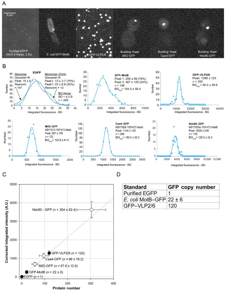
Biological questions are increasingly being addressed using a wide range of quantitative analytical tools to examine protein complex composition. Knowledge of the absolute number of proteins present provides insights into organization, function, and maintenance and is used in mathematical modeling of complex cellular dynamics. In this chapter, we outline and describe three microscopy-based methods for determining absolute protein numbers--fluorescence correlation spectroscopy, stepwise photobleaching, and ratiometric comparison of fluorescence intensity to known standards. In addition, we discuss the various fluorescently labeled proteins that have been used as standards for both stepwise photobleaching and ratiometric comparison analysis. A detailed procedure for determining absolute protein number by ratiometric comparison is outlined in the second half of this chapter. Counting proteins by quantitative microscopy is a relatively simple yet very powerful analytical tool that will increase our understanding of protein complex composition.
Keywords: Counting; FCS; Fluorescence; Fluorescence standards; Photobleaching; Quantitative imaging; Ratiometric.
© 2014 Elsevier Inc. All rights reserved.
Figures
Similar articles
-
Quantitative fluorescence microscopy and image deconvolution.Methods Cell Biol. 2013;114:407-26. doi: 10.1016/B978-0-12-407761-4.00017-8. Methods Cell Biol. 2013. PMID: 23931516
-
Counting protein molecules using quantitative fluorescence microscopy.Trends Biochem Sci. 2012 Nov;37(11):499-506. doi: 10.1016/j.tibs.2012.08.002. Epub 2012 Sep 2. Trends Biochem Sci. 2012. PMID: 22948030 Free PMC article. Review.
-
Quantitative fluorescence microscopy techniques.Methods Mol Biol. 2009;586:117-42. doi: 10.1007/978-1-60761-376-3_6. Methods Mol Biol. 2009. PMID: 19768427
-
Quantitative measurement of intracellular protein dynamics using photobleaching or photoactivation of fluorescent proteins.Microscopy (Oxf). 2014 Dec;63(6):403-8. doi: 10.1093/jmicro/dfu033. Epub 2014 Sep 28. Microscopy (Oxf). 2014. PMID: 25268018 Review.
-
Localization and mobility of bacterial proteins by confocal microscopy and fluorescence recovery after photobleaching.Methods Mol Biol. 2007;390:3-15. doi: 10.1007/978-1-59745-466-7_1. Methods Mol Biol. 2007. PMID: 17951677
Cited by
-
The interplay between BAX and BAK tunes apoptotic pore growth to control mitochondrial-DNA-mediated inflammation.Mol Cell. 2022 Mar 3;82(5):933-949.e9. doi: 10.1016/j.molcel.2022.01.008. Epub 2022 Feb 3. Mol Cell. 2022. PMID: 35120587 Free PMC article.
-
DNA-Origami-Based Fluorescence Brightness Standards for Convenient and Fast Protein Counting in Live Cells.Nano Lett. 2020 Dec 9;20(12):8890-8896. doi: 10.1021/acs.nanolett.0c03925. Epub 2020 Nov 9. Nano Lett. 2020. PMID: 33164530 Free PMC article.
-
Overexpression of Mdm36 reveals Num1 foci that mediate dynein-dependent microtubule sliding in budding yeast.J Cell Sci. 2020 Oct 15;133(20):jcs246363. doi: 10.1242/jcs.246363. J Cell Sci. 2020. PMID: 32938686 Free PMC article.
-
The relative binding position of Nck and Grb2 adaptors impacts actin-based motility of Vaccinia virus.Elife. 2022 Jul 7;11:e74655. doi: 10.7554/eLife.74655. Elife. 2022. PMID: 35796545 Free PMC article.
-
Quantitative mapping of fluorescently tagged cellular proteins using FCS-calibrated four-dimensional imaging.Nat Protoc. 2018 Jun;13(6):1445-1464. doi: 10.1038/nprot.2018.040. Epub 2018 May 24. Nat Protoc. 2018. PMID: 29844523 Free PMC article.
References
-
- Aravamudhan P, Felzer-Kim I, Joglekar AP. The budding yeast point centromere associates with two Cse4 molecules during mitosis. Current Biology. 2013;23(9):770–774. http://dx.doi.org/10.1016/j.cub.2013.03.042. - DOI - PMC - PubMed
-
- Bacia K, Schwille P. A dynamic view of cellular processes by in vivo fluorescence auto- and cross-correlation spectroscopy. Methods. 2003;29(1):74–85. - PubMed
-
- Braeckmans K, Deschout H, Demeester J, De Smedt SC. Optical fluorescence microscopy: From the spectral to the nano dimension. Berlin, Heidelberg: Springer-Verlag; 2011. Measuring molecular dynamics by FRAP, FCS, and SPT; pp. 153–163.
-
- Bulseco DA, Wolf DE. Fluorescence correlation spectroscopy: Molecular complexing in solution and in living cells. Methods in Cell Biology. 2013;114:489–524. http://dx.doi.org/10.1016/B978-0-12-407761-4.00021-X. - DOI - PubMed
-
- Charpilienne A, Nejmeddine M, Berois M, Parez N, Neumann E, Hewat E, et al. Individual rotavirus-like particles containing 120 molecules of fluorescent protein are visible in living cells. The Journal of Biological Chemistry. 2001;276(31):29361–29367. http://dx.doi.org/10.1074/jbc.M101935200. - DOI - PubMed
MeSH terms
Substances
Grants and funding
LinkOut - more resources
Full Text Sources
Other Literature Sources
