Prospects for building large timetrees using molecular data with incomplete gene coverage among species

Abstract

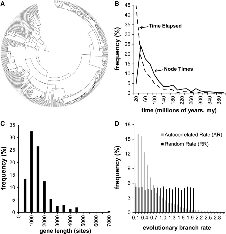
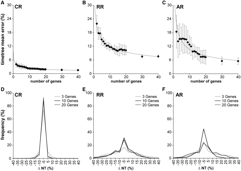
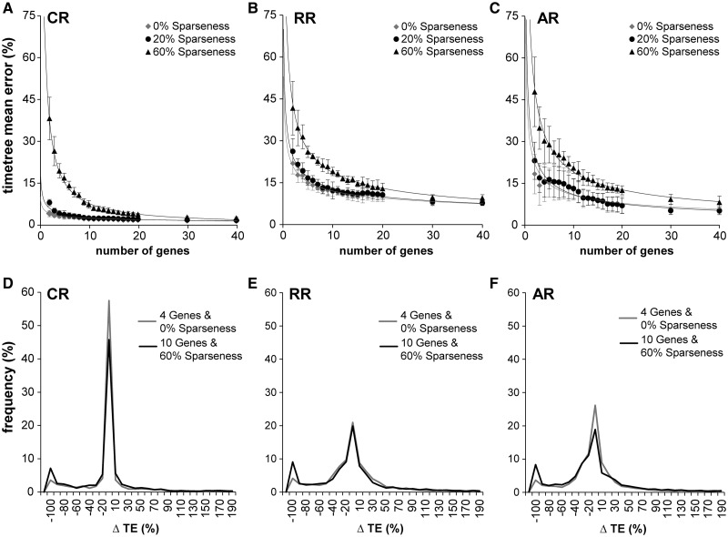
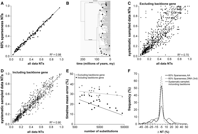
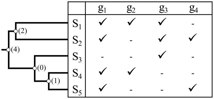
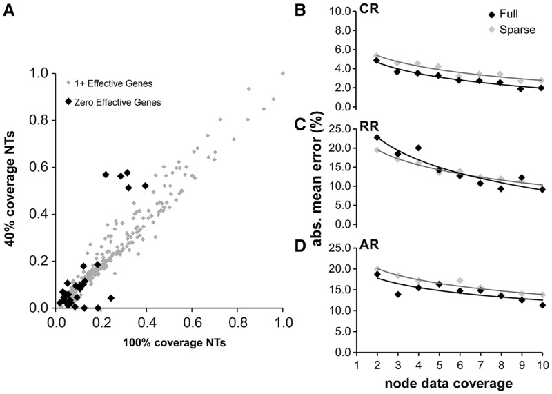
Scientists are assembling sequence data sets from increasing numbers of species and genes to build comprehensive timetrees. However, data are often unavailable for some species and gene combinations, and the proportion of missing data is often large for data sets containing many genes and species. Surprisingly, there has not been a systematic analysis of the effect of the degree of sparseness of the species-gene matrix on the accuracy of divergence time estimates. Here, we present results from computer simulations and empirical data analyses to quantify the impact of missing gene data on divergence time estimation in large phylogenies. We found that estimates of divergence times were robust even when sequences from a majority of genes for most of the species were absent. From the analysis of such extremely sparse data sets, we found that the most egregious errors occurred for nodes in the tree that had no common genes for any pair of species in the immediate descendant clades of the node in question. These problematic nodes can be easily detected prior to computational analyses based only on the input sequence alignment and the tree topology. We conclude that it is best to use larger alignments, because adding both genes and species to the alignment augments the number of genes available for estimating divergence events deep in the tree and improves their time estimates.

Keywords: divergence time; incomplete data; timetree.

Fig. 1.

Model tree and substitution patterns. (A) A 446-taxa phylogeny used for computer simulations. (B) Distribution of node divergence times (solid line) in the tree. The dashed line represents the distribution of elapsed time along branches of the tree. (C) Distribution of simulated gene alignment length, based on empirically observed gene lengths. (D) Rates were varied in the simulations to span a variety of models and evolutionary patterns. Because we generally do not have knowledge of actual rate variation patterns in real situations, we used three types of simulated evolutionary rate variation: As a baseline, a CR scenario, one in which the rate variation among branches was autocorrelated (AR), and one in which the (expected) evolutionary rates varied independently on each branch based on a uniform distribution, as described in Materials and Methods. A histogram is shown of the distribution of simulated rates in each case, with the nominal rate set equal to 1.0. In the CR case, the length distribution would be represented by a single bin at x = 1.0.

Fig. 2.

Error of divergence time estimates with increasing number of genes. Error (ΔNT) is measured as 100 × (H_EST − H_TRUE)/H_TRUE, where H_TRUE and H_EST are the true and estimated node heights (divergence times), respectively. (A–C) The mean estimation error for the entire tree by number of genes used for the different rate variation models. Error bars correspond to the standard deviation estimated from five replicates, each from a different sample of genes and rate assignments. In the CR case, only two genes are needed to achieve an average error of less than 5%. We used two additional, variable-rate models for sequence generation, RR and AR. In both of these cases, over 40 genes are needed to achieve a maximum average error of less than 5%, but only around 15 to bring error below 10%. (D–F) Distributions of the signed percentage divergence time estimation error of nodes for 1-, 3-, 10-, and 20-gene alignments. When more genes are used, the variance decreases, but a strong central tendency persists. In the CR and RR cases, there is little difference to be seen in the distributions between the 10- and 20-gene cases.

Fig. 3.

Effect of data sparseness on error. TE refers to time elapsed on a branch. (A–C) For each rate variation model and three different sparseness levels, the decline in error as more genes are added. In the CR case, there is virtually no difference between full data and 20% sparseness. 60% sparseness has considerably more error for fewer than ten genes, but as the number of genes increases, the error also converges to the full data levels. The RR situation is very similar but with error generally elevated over the CR case. AR shows a somewhat more pronounced difference between the full data and the 60% sparseness cases. (D–F) In these panels, we show the distributions of time estimate errors not for nodes, but for branches, in two cases, four genes with full data, and ten genes with 60% sparseness. In each case, there is the same number of sequences and taxa. We see that the distributions are virtually identical within each rate class, except for the left tail (−100% error case). These are cases in which the estimated branch lengths are zero. These are branches associated with nodes with zero data coverage (no genes with species in common to both child clades of the node). Such nodes have a substantial effect on mean error, but they can be easily detected a priori.

Fig. 4.

Results for amino acid divergence-time analyses of the 21-locus empirical data set of Meredith et al. (; see Materials and Methods for details). NT refers to relative time estimates of node divergence times. (A) Time estimate scatter diagram for analysis using the full set of 21 genes with 60% sparseness. In this case, because true divergence times are unknown, truth is taken to be the full-coverage case with all data. The R² coefficient of determination is 0.98. (B) Depiction of the mammalian clades used for the systematic sampling. Nineteen of the clades are marked by black diamonds, and the 20th is taken to be all of the remaining taxa. Each gene contains sequences for exactly two orders, assigned so that for each gene g₀, there exists exactly one gene g₁ and another gene g₂ such that g₀ shares exactly one clade with g₁ and the other clade with g₂. In this case, there is strictly limited species overlap among genes. We then added one “backbone” gene with a sequence for each taxon. The phylogenetic tree in the figure is based on the one that appears in Meredith et al. (2011). (C) Time estimate scatter diagram for analysis under the systematic sampling method described in the text, but without inclusion of the universal “backbone” gene. Again, truth is taken to be the full-coverage case with all data. (D) Time estimate scatter diagram for analysis under the systematic sampling method described in the text but in this case with the universal backbone gene. Resultant sparseness (percentage gaps in the data matrix) is approximately 90%. As before, truth is taken to be the full-coverage case with all data. We see that the R² coefficient (0.9) is much higher than in the case without backbone (0.7). (E) Effect of evolutionary rate of backbone gene on mean divergence time estimation error. Our mammalian data set contained 21 genes, each of which was used in turn as a backbone gene (black markers in the graph). The x axis represents the total number of substitutions observed for that gene and the y axis represents the total error of the resulting time tree. Gray markers represent 20-gene data sets without the backbone gene for each case (x value). Regression lines are fit to both sets of results and have R² values of 0.1 and 0.4 for the no-backbone and backbone case, respectively. We see that the use of the backbone gene is effective in reducing error and that faster-evolving backbone genes tend to be more effective than slowly evolving ones. (F) Distribution of signed error in the 60% sparse case when compared with the systematically sampled case with backbone. As we might expect from the fact that the systematic case is effectively 90% sparse, we see more spread to higher error in that case.

Fig. 5.

Node data coverage. The data coverage for any node in the phylogenetic tree is the number of genes that directly contribute to the time estimation for that node. A gene is considered to contribute to time estimation for a given node if it has sequences from at least one species pair, one each from the two immediate descendant clades. The figure shows a tree and corresponding data matrix, with genes g₁ to g₄ and species S₁ to S₅. Not all genes are available for each species. Available sequences are designated by check marks and missing ones are indicated by dashes in the matrix. Numbers in parentheses next to each node of the tree give the data coverage for that node. We may expect the time estimate for the node with zero data coverage to be very poor, since there is no sequence data to estimate the relevant branch length needed to estimate the divergence time. The best we can say is that it diverged at some time before either of its child nodes but after its parent node.

Fig. 6.

(A) A comparison of estimated divergence times based on ten genes and 60% sparseness is shown (RR rate model, other rate models give similar results). Nodes with zero data coverage are shown in black and have branch length time estimates of zero. These nodes are mostly shallow and have only a few species with data below them. (B–D) Relation between mean absolute value node time error and node data coverage for sparse (ten genes, 60% sparseness) and full coverage (zero sparseness, number of genes = node data coverage) in the CR, RR, and AR cases. The x axis is the node support and the y axis is the mean absolute value error for nodes with that amount of support. We see that, controlling for individual node support, there is very little, if any, difference in error between nodes in a sparse-coverage data set and in the full-coverage context.

References

1. Battistuzzi FU, Filipski A, Hedges SB, Kumar S. Performance of relaxed-clock methods in estimating evolutionary divergence times and their credibility intervals. Mol Biol Evol. 2010;27:1289–1300. - PMC - PubMed
1. Brown R, Yang Z. Rate variation and estimation of divergence times using strict and relaxed clocks. BMC Evol Biol. 2011;11:271. - PMC - PubMed
1. Cracraft J, Donoghue MJ. Assembling the tree of life. New York: Oxford University Press; 2004.
1. Douzery EJP, Delsuc F, Philippe H. Les datations moléculaires à l’heure de la génomique. Med Sci. 2006;22:374–380. - PubMed
1. Douzery EJP, Snell EA, Bapteste E, Delsuc F, Philippe H. The timing of eukaryotic evolution: does a relaxed molecular clock reconcile proteins and fossils? Proc Natl Acad Sci U S A. 2004;101:15386–15391. - PMC - PubMed
Publication types