Functional specialization in rat occipital and temporal visual cortex

Abstract

Recent studies have revealed a surprising degree of functional specialization in rodent visual cortex. Anatomically, suggestions have been made about the existence of hierarchical pathways with similarities to the ventral and dorsal pathways in primates. Here we aimed to characterize some important functional properties in part of the supposed "ventral" pathway in rats. We investigated the functional properties along a progression of five visual areas in awake rats, from primary visual cortex (V1) over lateromedial (LM), latero-intermediate (LI), and laterolateral (LL) areas up to the newly found lateral occipito-temporal cortex (TO). Response latency increased >20 ms from areas V1/LM/LI to areas LL and TO. Orientation and direction selectivity for the used grating patterns increased gradually from V1 to TO. Overall responsiveness and selectivity to shape stimuli decreased from V1 to TO and was increasingly dependent upon shape motion. Neural similarity for shapes could be accounted for by a simple computational model in V1, but not in the other areas. Across areas, we find a gradual change in which stimulus pairs are most discriminable. Finally, tolerance to position changes increased toward TO. These findings provide unique information about possible commonalities and differences between rodents and primates in hierarchical cortical processing.

Keywords: high-level vision; population coding; position tolerance; rodent research; single-unit recordings.

Fig. 1.

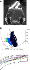
Localization of electrode tracks. A: representative coronal section of a CT scan of rat skull at the location of the craniotomy and recording chamber implant (7.9 mm caudal from bregma), showing the position of the craniotomy and the predicted electrode track. Scale bar, 1 mm. B, top: schematic overview of V1 and lateral extrastriate regions in the rat, based on the electrophysiological maps of Espinoza and Thomas (1983) and Thomas and Espinoza (1987). Red arrow represents the schematic anteroposterior location of our electrode tracks in relation to the different extrastriate areas: lateromedial (LM), latero-intermediate (LI), laterolateral (LL), and lateral occipito-temporal cortex (TO). Bottom: schematic overview of the relative position of the different electrode tracks (as derived from histology) within our 6 animals (animals A–F; each animal is differently colored) plotted on a schematic coronal slice (see Fig. 3B), indicating depth distribution of our tracks within the visual cortex. Note that many penetrations were performed in the animals, much more than the number of tracks that can be individuated from histology (most likely because most penetrations fall along the same line, as intended by the experimenter).

Fig. 2.

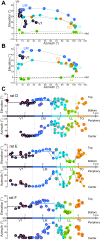
Retinotopy of visual areas. A and B: retinotopic location of neuronal receptive field (RF) centers along a single representative electrode track. Manually located RF centers illustrate the shift in azimuth with distance from entry point for each area. Neurons were located ∼100 μm apart. Numbers in circles correspond to the order in which the neurons were recorded. Color coding of circles indicates the area to which these neurons were assigned based on retinotopic progression and mirroring. VM, vertical meridian; HM, horizontal meridian. Note the spherical correction that causes flat screen coordinates to appear vertically compressed at high azimuth. C: detailed representation of retinotopic changes along electrode tracks for 3 representative rats show different elevations as well as mirroring of azimuth in each area. For each rat the elevation (above bar) and azimuth (below bar) of the RF center are plotted relative to the distance from the entry point. Since entry point position often slightly shifted with the number of penetrations because of brain damage just below the craniotomy, distances from entry point were further calibrated by aligning the observed border between LL and TO or, if this border was not sampled, between LM and LI. These borders were always marked by a sharp mirroring of the retinotopy at the far periphery and a shift in elevation over a short distance. Each circle indicates the RF center elevation and azimuth of each cell recorded in these animals. RF center position was determined either manually (colored circles, as in A and B) or automatically by determining the center of gravity of the optimal response positions on the screen (colored circles with red outline). Cells recorded during the same penetration carry identical letters. Penetrations are labeled chronologically in alphabetical order. Cells recorded during penetrations that provided the largest numbers of recorded cells and enabled us to clearly determine the retinotopy are connected by black lines in the order in which the units were recorded. Color of the unit circles represents areal identity as determined during the penetration based on position of this RF as well as population RFs of sites that were briefly assessed but not formally recorded from with the various experiments. Thick lines in the elevation plots indicate mean elevation for each area. Gray dashed lines represent areal borders. The line between the elevation and azimuth plots represents a schematic representation of the different areas along our electrode tracks. Color coding for each area is identical to that used in subsequent figures.

Fig. 3.

Immunohistochemistry along electrode tracks. A: section immunostained for Neurofilament protein from the animal in Fig. 1A, illustrating the position of the electrolytic lesion made at the end of our last electrode penetration. On the basis of the responses recorded during this last penetration we estimated the lesion to be 500 μm beyond the lateral border of area TO. Scale bar, 1 mm. B: detail of Neurofilament protein-labeled section from A (top) and adjacent Nissl-stained section (bottom) clearly show the location of 1 of the lesions. Functionally defined areal borders are indicated by white arrowheads along the reconstructed electrode track, while anatomically defined interareal borders between V1 and LM and LL and Te2d are indicated by black arrowheads at the cortical surface (see materials and methods for details). Scale bar, 500 μm.

Fig. 4.

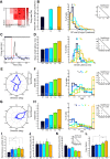
Simple and complex cells in rat V1 and eye movements. A: example peristimulus time histogram (PSTH) of a simple cell in V1 [modulation of the response (F₁)/net firing rate (F₀) = 1.16], responding to a drifting grating of optimal orientation. Black and white bars indicate that the stimulus is off or on, respectively. B: frequency distribution of F₁/F₀ of V1 neurons (n = 160). C: example eye movement trace, showing the distance in degrees between the pupil center and the median pupil position. Stimulus onset and offset (experiment 5, shapes at 2 different positions, indicated as blue and red bars) are plotted below the trace, showing that there is no correlation between eye movements and stimulus position. Eye movements were very small compared with the distance between the 2 stimulus positions (right y-axis). About 79% of this trace falls within 1.25° from the central position, which is slightly above the overall average of 75% (see inset).

Fig. 5.

Population data of neuronal response properties. A: color-coded responses of a representative LI neuron to a static shape at 15 different screen positions. Asterisks indicate positions where the neuron produced a statistically significant response (t-test, Bonferroni corrected for multiple comparisons); the black dot defines the position of the neuron's center of gravity weighted for firing rate at the significant positions. B: population data of RF size (no. of screen positions eliciting a significant response) in V1, LI, and TO. C: PSTH of the response of a representative neuron to static shapes (experiment 3). Red line indicates stimulus onset; stimulus remains on the screen during the rest of the PSTH. Solid blue line represents mean baseline response; dashed line represents mean baseline response + 3 SDs. Red triangle indicates onset latency, defined as the time after stimulus onset where the histogram crosses this threshold. D: neuronal population data of onset latency in all visual areas. E and G: representative tuning curves for stimulus direction for an orientation (E)- and a direction (G)-selective cell. F and H: population data of orientation selectivity index (OSI, F) and direction selectivity index (DSI, H) in all visual areas. B, D, F, and H: bar graphs on left show mean of the response property for each area and error bars indicate SE. Center: frequency distributions of the response property for all neurons in each area. Colors indicate area and are matched with those in the bar graphs. Closed triangles represent the mean and open diamonds the medians of the population response property. Right: statistical significance of pairwise comparisons of median response property (Wilcoxon signed-rank test) for each visual area (*P < 0.05, Bonferroni corrected for multiple comparisons). I–L: median values of spontaneous activity (I), maximal raw firing rate (J), maximal net firing rate (K), and Fano factor (L) in all areas obtained during the orientation tuning experiment (C–F). Error bars indicate confidence intervals. *Statistical significance (Wilcoxon signed-rank test as above).

Fig. 6.

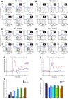
Static shapes elicit little sustained response in higher areas. A–D: single-unit responses to static and moving shapes. For static shapes, we show the raster plots for the whole 500-ms stimulus presentation; for moving shapes, we show the comparable window of the first 500 ms of the full 4,000-ms presentation duration. Vertical green line indicates stimulus onset. Horizontal black lines indicate average baseline firing rate (200 ms preceding stimulus onset); horizontal red lines indicate average firing rate during the 500-ms interval after stimulus onset. The number of trials varied for static shapes between 25 and 26 and for moving shapes between 12 and 13. Example neurons are the same as shown in Fig. 7. The example V1 neuron shows strong responses to static (A) and moving (C) shapes. The example TO neuron (B and D) shows little sustained response to static shapes, except for an initial transient, and a more sustained and selective response to moving shapes. E and F: comparison of average traces in response to static or moving stimuli in V1 (E) and highest area, TO (F). G: normalized sustained response to static and moving shapes in the different areas, averaged across all neurons (error bars indicate SE). H: SVM classifier performances when using data for moving and static shapes; equal intervals (500 ms) were used to calculate response rates. Red bars indicate threshold for significance of individual bars. Asterisks indicate significant differences between bars, calculated by shuffling experiment labels.

Fig. 7.

Responses of 2 representative neurons from V1 (A) and TO (B) to moving shapes at 2 different positions. PSTH and raster plots are shown on left for the shapes with the highest and lowest responses at the first position (top) and the same shapes at the second position (bottom). Horizontal black lines indicate average baseline firing rate (1 s preceding stimulus onset); horizontal red lines indicate average firing rate during the 4-s interval after stimulus onset. Right: net mean response rates for all shapes at the first and second stimulus positions. Both neurons show selectivity at the best position, but only in TO do we observe tolerance for position. Insets: mean spike waveforms.

Fig. 8.

Population data of single-unit indicators of shape selectivity. A–D: median values of spontaneous activity (A), maximal raw firing rate (B), maximal net firing rate (C), and Fano factor (D) in all areas obtained during the presentation of moving shapes (see Fig. 7). E: median ratio of net response rates for the shape with maximal response rate over the mean net response rate of all shapes. F: frequency distribution of maximum-to-mean response ratio. G: median response sparseness for the 6 different shapes. H: frequency distribution of response sparseness. Error bars in A–E and G indicate confidence intervals. *Statistical significance (Wilcoxon signed-rank test P < 0.05, Bonferroni corrected for multiple comparisons). F and H, left: closed triangles represent the mean and open diamonds the medians of the population response property. Right: statistical significance of pairwise comparisons of median response property (Wilcoxon signed-rank test) for each visual area (*P < 0.05, Bonferroni corrected for multiple comparisons).

Fig. 9.

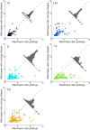
Relation between selectivity for oriented drifting gratings and shapes: comparison between max-to-mean response ratios for drifting gratings vs. moving shapes for the 5 visual areas. Histograms indicate the difference in the max-to-mean response ratios between moving shapes and drifting gratings. In most areas max/mean, i.e., the selectivity for the different stimuli, was higher for the drifting gratings than for the shapes.

Fig. 10.

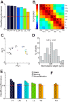
Gradual change in information readout over different areas. A: SVM classifier pairwise discrimination performance (averaged across 15 shape pairs) per area, including upper and lower layers of V1 (V1U and V1L). Red lines indicate significance levels obtained through permutations. Dashed line indicates chance level. B: correlation matrix based on dissimilarity scores for 15 shape pairs based on physical stimulus properties (Pix and V1s) and neural responses (in areas V1, LM, LI, LL, and TO and V1U and V1L). C: plot of the first 2 principal components computed for the correlation matrix shown in B. This representation indicates that upper layers of V1 are more similar to physical measures; lower layers code the shapes more like area LM, downstream to V1. D: depth distribution of neurons in orthogonal V1 penetrations for units used in V1U and V1L. Depth is normalized for small differences in electrode tilt. Dashed line indicates division between upper (V1U; left) and lower (V1L; right) layers. E: SVM classifier discrimination performance averaged over 15 shape pairs per area using the initial peak response (41–240 ms after stimulus onset) only. Left bars show discrimination performance for static stimuli, center bars show discrimination performance for moving stimuli, and right bars show the classifier generalization from static to moving stimuli, obtained after training the SVM classifier on responses to static shapes and testing this classifier on responses to the moving shape. Red lines indicate significance levels obtained through permutations. Dashed line indicates chance level. There is significant generalization from static to moving stimuli in all areas except for TO. In F we show the same generalization data for TO, but here only the responses in a 60-ms interval around the population PSTH peak were used. Significant generalization was observed.

Fig. 11.

Comparison between selectivity and tolerance. A: selectivity (colored bars, left) and tolerance (shaded bars, right) SVM classifier performance for V1, LM, LI, LL, and TO and V1U and V1L. Red lines indicate significance threshold based on permutations; asterisks indicate significant differences between selectivity and tolerance for the same area. B: ratio between selectivity and tolerance (data shown in A) for the same areas. The ratios are corrected for chance performance obtained when guessing. *Ratios differ significantly from 1. C: selectivity and tolerance SVM performance in V1 and TO for the subset of neurons that was equated for selectivity. Also in this subset there is a significantly higher tolerance in TO compared with V1. Black lines indicate average performance after shuffling area labels, and the gray area indicates the 95% confidence interval. *The observed difference between V1 and TO exceeds what is expected by chance. D: scatterplots of selectivity and tolerance SVM performance of all shape pairs. Triangles indicate mean SVM classifier performances as shown in A. E: single-unit measures of selectivity and tolerance. For different areas, the neural responses at both positions are shown, sorted according to preference at the first (most responsive) position (solid line). Responses of each population of neurons were normalized to have an average 1 for the best and 0 for the worst shapes at this position. Responses at the second position, sorted and normalized according to the responses at the first position, are indicated with a dashed line. Red lines show a linear fit through the data points for the second position.

References

1. Alemi-Neissi A, Rosselli FB, Zoccolan D. Multifeatural shape processing in rats engaged in invariant visual object recognition. J Neurosci 33: 5939–5956, 2013 - PMC - PubMed
1. Andermann ML, Kerlin AM, Roumis DK, Glickfeld LL, Reid RC. Functional specialization of mouse higher visual cortical areas. Neuron 72: 1025–1039, 2011 - PMC - PubMed
1. Brainard DH. The Psychophysics Toolbox. Spat Vis 10: 433–436, 1997 - PubMed
1. Braje WL, Kersten D, Tarr MJ, Troje NF. Illumination effects in face recognition. Psychobiology 26 371–380, 1998
1. Chelazzi L, Rossi F, Tempia F, Ghirardi M, Strata P. Saccadic eye movements and gaze holding in the head-restrained pigmented rat. Eur J Neurosci 1: 639–646, 1989 - PubMed
Publication types
LinkOut - more resources