Neurocognitive mechanisms of statistical-sequential learning: what do event-related potentials tell us?

Abstract

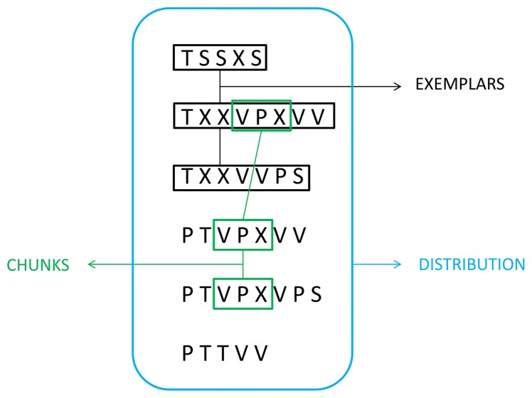
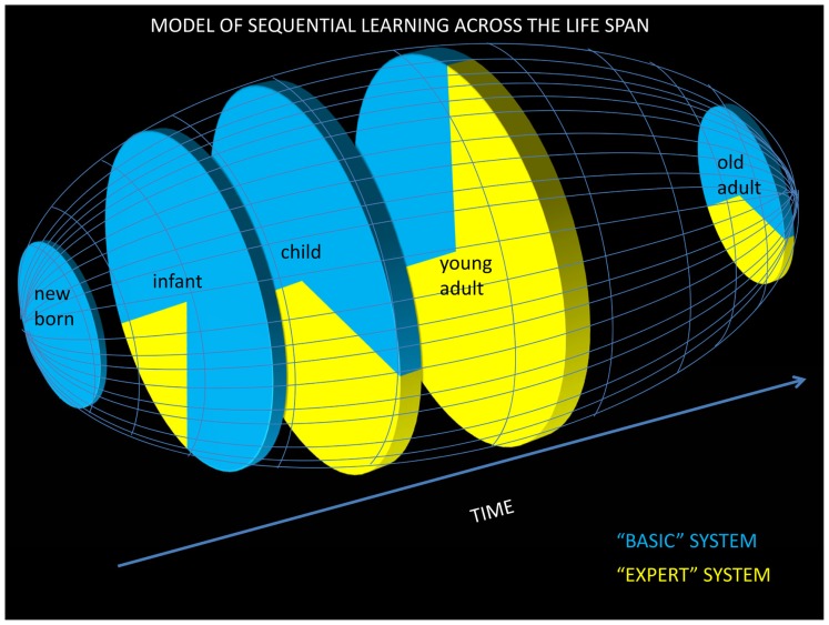
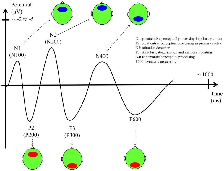
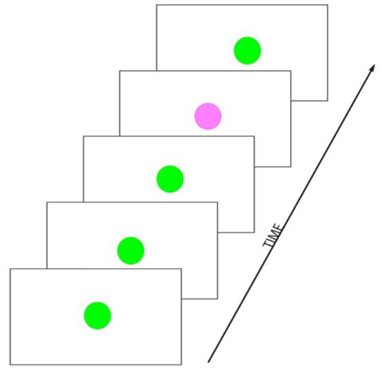
Statistical-sequential learning (SL) is the ability to process patterns of environmental stimuli, such as spoken language, music, or one's motor actions, that unfold in time. The underlying neurocognitive mechanisms of SL and the associated cognitive representations are still not well understood as reflected by the heterogeneity of the reviewed cognitive models. The purpose of this review is: (1) to provide a general overview of the primary models and theories of SL, (2) to describe the empirical research - with a focus on the event-related potential (ERP) literature - in support of these models while also highlighting the current limitations of this research, and (3) to present a set of new lines of ERP research to overcome these limitations. The review is articulated around three descriptive dimensions in relation to SL: the level of abstractness of the representations learned through SL, the effect of the level of attention and consciousness on SL, and the developmental trajectory of SL across the life-span. We conclude with a new tentative model that takes into account these three dimensions and also point to several promising new lines of SL research.

Keywords: ERP; P300; P600; artificial grammar; implicit learning; procedural learning; sequential learning; statistical learning.

FIGURE 1

Three types of concrete feature representations involved in encoding a sequence of letter strings generated from an artificial grammar (see “Artificial Grammar and Natural Language Paradigms” section): fragment-based or chunk information, exemplars, and distributional information (modified with permission from Cleeremans et al., 1998).

FIGURE 2

Model of SL across the life span. We propose that SL is governed by two systems: a “basic” and an “expert” system. The “basic” system incorporates modality-specific predictive mechanisms that are mostly automatic and implicit and that capture concrete structures of sequences such as chunks and transition probabilities through a bottom-up process. The basic system, which is possibly a sub-system (in the temporal domain) of the (spatio-temporal) PL system, can be modeled by simple recurrent networks. The “basic” system is already available very early in life, allowing for the development of explicit long-term associative memories that become available to the expert SL system. The “expert” system, which relies on top-down explicit multimodal and retrospective mechanisms, depends on the level of intention (to learn) and attention (including selective attention through social cues). The “expert” system, which captures more abstract patterns, increasingly develops from childhood into adulthood and then declines in old age because of impaired working and sensory memories. Blue represents the proportion of SL governed by the basic system and yellow represents the proportion of SL governed by the expert system. Clearly, this model is tentative and highly speculative. In particular, the exact degree of contribution of the basic and expert systems at different ages of life remain currently unknown.

FIGURE 3

Main ERP components with their functional interpretation, latencies, and scalp topography (ellipses indicate the scalp location where the component has the largest amplitude – red: positive potential, blue: negative potential; vertical axis unit: scalp potential in microvolts with negativity upward; horizontal axis unit: time from the stimulus onset in milliseconds).

FIGURE 4

Example of an oddball paradigm in the visual domain. Visual stimuli are presented in a temporal sequence. The green colored circle stimulus is frequently presented and is referred to as the “frequent” or “standard” stimulus. The pink colored circle is rarely presented and is referred to as the “rare” or “deviant” or “target” stimulus. The number of standards presented between two deviants is pseudo-random.

FIGURE 5

One possible depiction of the serial reaction time task ((Nissen and Bullemer, 1987). Visual stimuli appear at different – non-random – locations in a temporal sequence. Participants have to reproduce the displayed sequence by pressing on the touch screen at the correct locations and in the same temporal order as the displayed sequence. Note that the actual configuration of the stimulus locations can vary across studies.

FIGURE 6

Modified oddball paradigm of Jost et al. (2011). The standard stimulus is a white circle on a dark background. The paradigm comprises several deviant stimuli belonging to two different categories: “predictor” and “target”. Participants are asked to press a button when the target is presented. There are three types of predictors (corresponding to the three experimental conditions): a “high probability” predictor which is followed 90% of the trials by the target, a “low probability” predictor, followed 20% of the trials by the target, and a “zero probability” predictor, which is never followed by the target. Participants are not told about these predictor-target variable statistical contingencies. SL is observed behaviorally when performance improves with higher statistical contingency. SL is observed neurophysiologically when the ERP to the predictors differ between the experimental conditions (e.g., a larger amplitude for the high probability predictor compared to the other two predictor types).

FIGURE 7

Example of an artificial grammar in the visual domain. The algorithm describes the rules of the artificial grammar, that is the set of possible sequences of stimuli (in this case, colored squares) that are valid according the rules of the grammar. Examples of valid sequences (i.e., grammatical sequences containing no syntactic violations) are presented on the bottom of the figure circled in dark. Examples of non-grammatical sequences (containing syntactic violations) are also presented, circled in red.

FIGURE 8

Left panel: Mean response time to a SRT for grammatical (“Gram”) and ungrammatical (“Ungram”) sequences across practice sessions (each session lasts for four hours) under implicit (“IMP,” participants were not previously informed of the sequence structure) and explicit conditions (“EXP,” participants were previously informed of the sequence structure). Right panel: Difference waves (ERP to ungrammatical targets minus ERP to grammatical targets) under implicit and explicit conditions. (Reproduced with permission from Baldwin and Kutas, 1997).

FIGURE 9

Left panel: Mean response time difference to a SRT (RT to ungrammatical sequences minus RT to grammatical sequences) across practice sessions/blocks (each block consists of 120 trials with the presentation of 12 sequences of 10 letters) under implicit (“I,” participants who did not report noticing the presence of a sequence when asked after the experiment) and explicit conditions (“E,” participants who reported noticing the presence of a sequence when asked after the experiment). Right panel: Mean ERP amplitude in the 240–340 ms poststimulus onset time range (corresponding to the N2 component) to the deviant stimulus (ungrammatical sequences) minus ERP to the standard stimulus (grammatical sequences) under implicit (“I”) and explicit conditions (“E”) from the first and second halves of the blocks. (Reproduced with permission from Eimer et al., 1996).