Applying compressed sensing to genome-wide association studies

Abstract

Background: The aim of a genome-wide association study (GWAS) is to isolate DNA markers for variants affecting phenotypes of interest. This is constrained by the fact that the number of markers often far exceeds the number of samples. Compressed sensing (CS) is a body of theory regarding signal recovery when the number of predictor variables (i.e., genotyped markers) exceeds the sample size. Its applicability to GWAS has not been investigated.

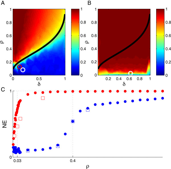
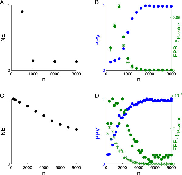
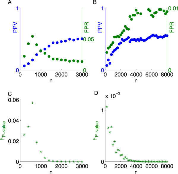
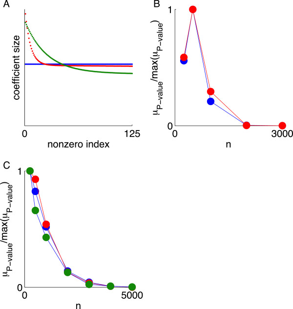
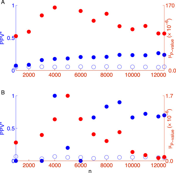
Results: Using CS theory, we show that all markers with nonzero coefficients can be identified (selected) using an efficient algorithm, provided that they are sufficiently few in number (sparse) relative to sample size. For heritability equal to one (h (2) = 1), there is a sharp phase transition from poor performance to complete selection as the sample size is increased. For heritability below one, complete selection still occurs, but the transition is smoothed. We find for h (2) ∼ 0.5 that a sample size of approximately thirty times the number of markers with nonzero coefficients is sufficient for full selection. This boundary is only weakly dependent on the number of genotyped markers.

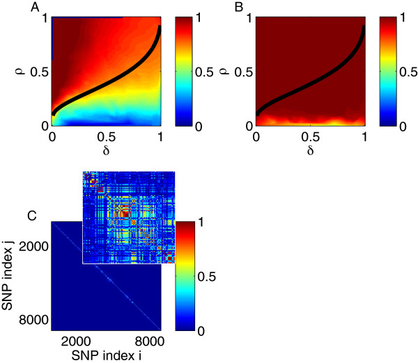
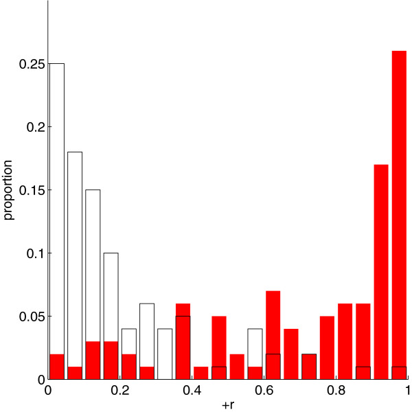
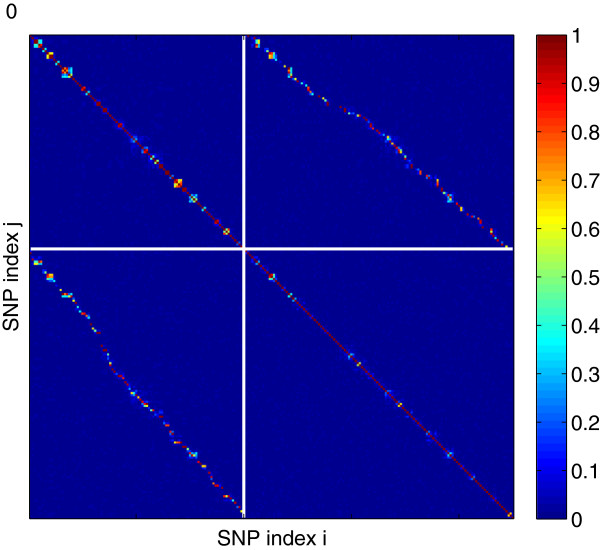
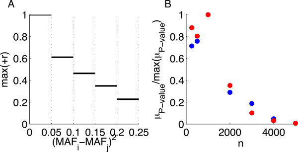
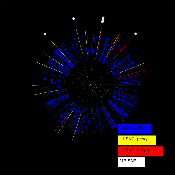
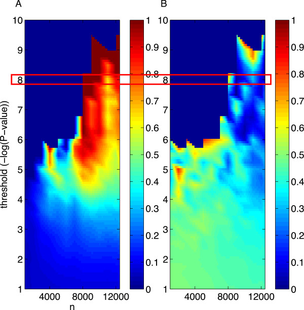
Conclusion: Practical measures of signal recovery are robust to linkage disequilibrium between a true causal variant and markers residing in the same genomic region. Given a limited sample size, it is possible to discover a phase transition by increasing the penalization; in this case a subset of the support may be recovered. Applying this approach to the GWAS analysis of height, we show that 70-100% of the selected markers are strongly correlated with height-associated markers identified by the GIANT Consortium.

Keywords: Compressed sensing; GWAS; Genomic selection; Lasso; Phase transition; Sparsity; Underdetermined system.

Figure 1

Error in the ρ − δ plane for a measurement matrix of random genomic SNPs ($\mathit{\rho }=\frac{\mathit{s}}{\mathit{n}}$ and $\mathit{\delta }=\frac{\mathit{n}}{\mathit{p}}$). (A) Color corresponds to the normalized error (NE) of the coefficients $\frac{{∥\mathit{x}-\widehat{\mathit{x}}∥}_{\mathit{L}2}}{{∥\mathit{x}∥}_{\mathit{L}2}}$. The black curve is the expected phase boundary between poor and good recovery from [26]. The number of SNPs, p, was fixed at 8,027. The heritability was set to one (noiseless case). The circles correspond to the points (ρ = 0.08, δ = 0.19) (white) and (ρ = 0.125, δ = 0.125) (red) discussed in Measures of selection. (B) Same as panel (A), except that the heritability was set to 0.5 (noisy case). The white circle corresponds to the point (ρ = 0.025, δ = 0.625) discussed in Measures of selection. (C)NE versus ρ for fixed n = 4,000 and p = 8,027 (blue corresponds to h² = 1, red to h² = 0.5). The square markers indicate recovery quality evaluated at a few data points using the lasso algorithm with 10-fold cross-validation written by MATLAB.

Figure 2

Measures of selection as a function of sample size for the measurement matrix of random genomic SNPs. Fixing s = 125 and p = 8,027, we measured the selection of true nonzero coefficients according to four metrics for h² = 1 (A-B) and h² = 0.5 (C-D). Shown in (A-C) is the normalized error of the coefficients (NE). Shown in (B-D) are the positive predictive value (PPV, blue dots), false positive rate (FPR, green dots), and median P -value (μ_{P − value}, green asterisks). The point n = 1, 000 corresponds to (ρ = 0.125, δ = 0.125) and n = 5, 000 to (ρ = 0.025, δ = 0.625) noted in Figure 1A and B respectively.

Figure 3

Analysis of chromosome 22. (A) The ρ − δ plane for h² = 1. p was set to 8,915. Superimposed is the expected phase boundary when there is neither noise nor LD [26]. (B) The same as panel (A), except for h² = 0.5. (C) The matrix of correlations (positive roots of the r² LD measure) between genotyped SNPs on chromosome 22. Inset is a 100 × 100 sample along the diagonal.

Figure 4

Measures of selection as a function of sample size for chromosome 22 (s = 125 and p = 8, 915). The PPV (blue) and FPR (green) for h² = 1 (A) and h² = 0.5 (B). μ_{P − value} for h² = 1 (C) and h² = 0.5 (D).

Figure 5

Distribution of maximum correlations between false positives and true nonzeros after the presumptive μ_{P − value}phase transition for chromosome 22. Histogram of the maximum correlation (maximum of the positive roots of the r² LD measure) between a false positive and true nonzero for chromosome 22, given s = 125, n = 5,000, and h² = 0.5 (red). Also shown is one realization from the null distribution, generated by drawing an equal number of “false positives” at random from chromosome 22 (white).

Figure 6

The matrix of correlations (positive roots of the r² LD measure) among false positives and true nonzeros after the presumptive μ_{P − value}phase transition for chromosome 22 (s = 125, n = 5, 000, and h² = 0.5). SNP indices begin at the top left corner. The upper-left quadrant contains the correlations among false positives and the lower-right quadrant contains the correlations among the true nonzeros. Each element in the upper-right (lower-left) quadrant represents a correlation between a false positive and a true nonzero. Within both the false positive and the true nonzero sets, the markers are arranged in order of chromosomal map position.

Figure 7

Insensitivity of the selection phase boundary to the distribution of coefficient magnitudes (ensemble). (A)s = 125 coefficient magnitudes (“effect sizes”) ordered from large to small for the Uniform (blue), Hyperexponential 1 (red), and Hyperexponential 2 (green) ensembles. (B) Chromosome 22 analysis using μ_{P − value} to measure selection (normalized by the maximum value) as a function of sample size for h² = 1 for the Uniform (blue) and Hyperexponential 1 (red) ensembles. (C) As in panel (B) except for h² = 0.5. Also shown is recovery for the Hyperexponential 2 ensemble (green).

Figure 8

Insensitivity of the selection phase boundary to minor allele frequency (MAF) for chromosome 22. (A) The maximum positive root of the r² LD measure (+r) as a function of squared MAF difference. The maxima are estimated over bin lengths of 0.05 for SNPs in chromosome 22. (B) The median P -value (μ_{P − value}) normalized by the maximum value as a function of sample size for s = 125 from {−1,  1} and h² = 0.5 for nonzero coefficients sampled from low (blue) or high (red) MAF SNPs on chromosome 22.

Figure 9

Selection measures as a function of sample size in an analysis of real height data. (A) The adjusted positive predictive value (PPV*, blue solid dots) and median P -value (μ_{P − value}, red) as a function of sample size using λ based on h² = 0.5. Also shown is PPV* when the same number of SNPs are randomly selected rather than returned by the L₁ algorithm (blue unfilled dots). (B) As in (A) but setting λ to a value appropriate for h² = 0.01.

Figure 10

Map of SNPs associated with height, as identified by the GIANT Consortium meta-analysis, L₁ -penalized regression, and standard GWAS. Base-pair distance is given by angle, and chromosome endpoints are demarcated by dotted lines. Starting from 3 o’clock and going counterclockwise, the map sweeps through the chromosomes in numerical order. As a scale reference, the first sector represents chromosome 1 and is ∼ 250 million base-pairs. The blue segments correspond to a 1 Mb window surrounding the height-associated SNPs discovered by GIANT. Note that some of these may overlap. The yellow segments represent L₁ -selected SNPs that fell within 500 kb of a (blue) GIANT-identified nonzero; these met our criterion for being declared true positives. The red segments represent L₁ -selected SNPs that did not fall within 500 kb of a GIANT-identified nonzero. Note that some yellow and red segments overlap given this figure’s resolution. There are in total 20 yellow/red segments, representing L₁ -selected SNPs found using all 12,454 subjects. The white dots represent the locations of SNPs selected by MR at a P -value threshold of 10^− 8.

Figure 11

Measures of recovery using marginal regression (standard GWAS) as a function of sample size. All SNPs surviving the chosen − log₁₀P − value threshold were selected. The recovery measures, computed over the selected SNPs, were (A) the adjusted positive predictive value (PPV*) and (B) the median P -value divided by the P -value cutoff. Highlighted in red is the cutoff we used for MR in Figure 10.

References

1. Johnstone IM, Titterington DM. Statistical challenges of high-dimensional data. Philos Trans R Soc A. 2009;367:4237–4253. doi: 10.1098/rsta.2009.0159. - DOI - PMC - PubMed
1. Hoggart CJ, Whittaker JC, De Iorio M, Balding DJ. Simultaneous analysis of all SNPs in genome-wide and re-sequencing association studies. PLoS Genet. 2008;4:e1000130. doi: 10.1371/journal.pgen.1000130. - DOI - PMC - PubMed
1. Goddard ME, Wray NR, Verbyla K, Visscher PM. Estimating effects and making predictions from genome-wide marker data. Stat Sci. 2009;24:517–529. doi: 10.1214/09-STS306. - DOI
1. Kemper KE, Daetwyler HD, Visscher PM, Goddard ME. Comparing linkage and association analyses in sheep points to a better way of doing GWAS. Genet Res. 2012;94:191–203. doi: 10.1017/S0016672312000365. - DOI - PubMed
1. Genovese CR, Jin J, Wasserman L, Yao Z. A comparison of the lasso and marginal regression. J Mach Learn Res. 2012;13:2107–2143.