Granger causality revisited

Abstract

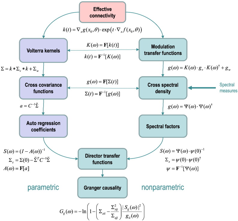
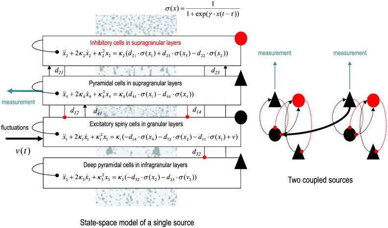
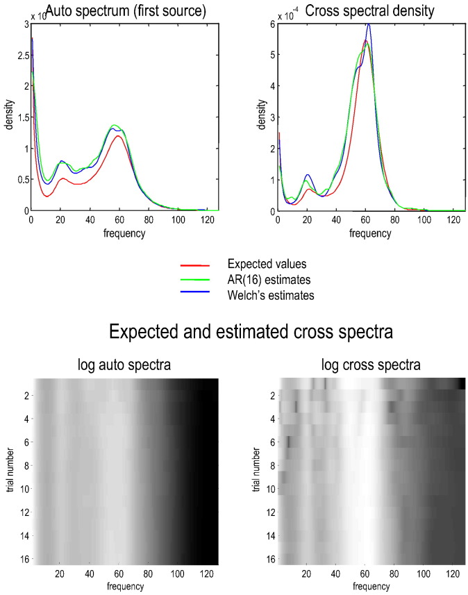
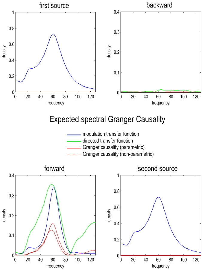
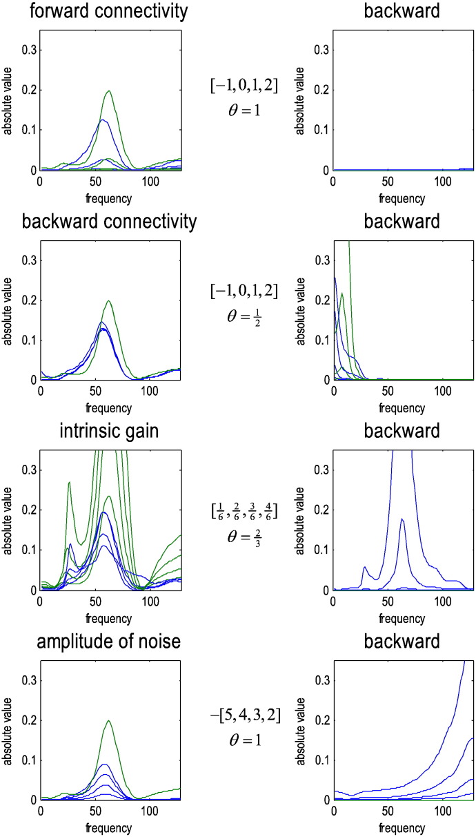
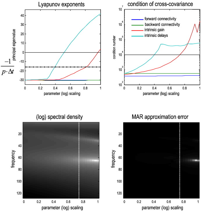
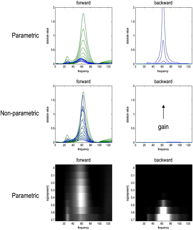
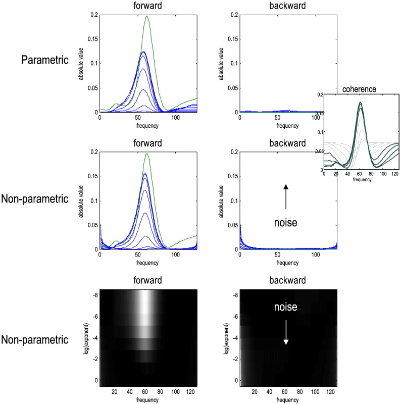
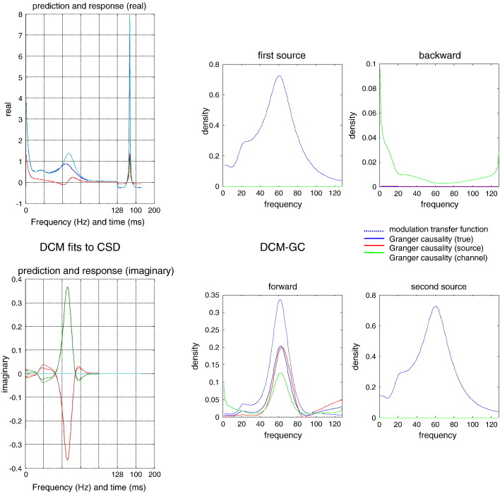
This technical paper offers a critical re-evaluation of (spectral) Granger causality measures in the analysis of biological timeseries. Using realistic (neural mass) models of coupled neuronal dynamics, we evaluate the robustness of parametric and nonparametric Granger causality. Starting from a broad class of generative (state-space) models of neuronal dynamics, we show how their Volterra kernels prescribe the second-order statistics of their response to random fluctuations; characterised in terms of cross-spectral density, cross-covariance, autoregressive coefficients and directed transfer functions. These quantities in turn specify Granger causality - providing a direct (analytic) link between the parameters of a generative model and the expected Granger causality. We use this link to show that Granger causality measures based upon autoregressive models can become unreliable when the underlying dynamics is dominated by slow (unstable) modes - as quantified by the principal Lyapunov exponent. However, nonparametric measures based on causal spectral factors are robust to dynamical instability. We then demonstrate how both parametric and nonparametric spectral causality measures can become unreliable in the presence of measurement noise. Finally, we show that this problem can be finessed by deriving spectral causality measures from Volterra kernels, estimated using dynamic causal modelling.

Keywords: Cross spectra; Dynamic causal modelling; Dynamics; Effective connectivity; Functional connectivity; Granger causality; Neurophysiology.

Fig. 1

This schematic illustrates the different routes one could take – using the equations in Table 1 – to derive (spectral) Granger causality measures from the (effective connectivity) parameters of a model — or indeed empirical measures of cross spectral density. The key point made by this schematic is the distinction between parametric and nonparametric spectral causality measures. These both rest upon the proportion of variance explained, implicit in the directed transfer functions; however, in the parametric form, the transfer functions are based upon an autoregression model. In contrast, the nonparametric approach uses spectral matrix factorisation, under the constraint that the spectral factors are causal or minimum phase filters. The boxes in light green indicate spectral characterisations, while the light blue boxes indicate measures in the time domain. See Table 1 and main text for a more detailed explanation of the variables and operators.

Fig. 2

This schematic illustrates the state-space or dynamic causal model that we used to generate expected cross spectra and simulated data. Left panel: this shows the differential equations governing the evolution of depolarisation in four populations constituting a single electromagnetic source (of EEG, MEG or LFP measurements). These equations are expressed in terms of second-order differential equations that can be rewritten as pairs of first order equations, which describe postsynaptic currents and depolarisation in each population. These populations are divided into input cells in granular layers of the cortex, inhibitory interneurons and (superficial and deep) principal or pyramidal cell populations that constitute the output populations. The equations of motion are based upon standard convolution models for synaptic transformations, while coupling among populations is mediated by a sigmoid function of (delayed) mean depolarisation. The slope of the sigmoid function corresponds to the intrinsic gain of each population. Intrinsic (within-source) connections couple the different populations, while extrinsic (between-source) connections couple populations from different sources. The extrinsic influences (not shown) enter the equations in the same way as the intrinsic influences but in a laminar specific fashion (as shown in the right panel). Right panel: this shows the simple two source architecture used in the current paper. This comprises one lower source that sends forward connections to a higher source (but does not receive reciprocal backward connections). The intrinsic connectivity (dotted lines) and extrinsic connectivity (solid line) conform to the connectivity of the canonical microcircuit and the known laminar specificity of extrinsic connections (Bastos et al., 2012). Excitatory connections are in red and inhibitory connections are in black. Random fluctuations drive the input cells and measurements are based on the depolarisation of superficial pyramidal cells. See Table 2 for a list of key parameters and a brief description.

Fig. 3

This figure illustrates the convergence of empirical estimates of spectral density averaged over multiple trials. The top row shows the absolute values of the auto (for the first source) and cross spectral density (between the two sources of Fig. 2). The red lines correspond to the expected spectra under the known parameters of the model (the parameters used for characterising spectral measures in subsequent figures). The green and blue lines correspond to empirical estimates based upon 16 epochs of simulated (noisy) data, where each epoch comprised 1024 samples at a sampling rate of 256 Hz. The green lines report the estimates under an AR(16) model, while the blue lines used Welch's periodiogram method, as implemented in Matlab. Both give very similar results. The lower panels show the (absolute value) of the emerging average over 16 trials to show that stable estimates obtain after about eight trials — although many more are generally used in practice to obtain smooth spectral estimates.

Fig. 4

This figure reports the expected modulation transfer functions (blue lines), normalised directed transfer functions (green lines) and the associated spectral Granger causality (red lines: parametric — solid and nonparametric — dotted) under the dynamic causal model shown in Fig. 1. In this example, measurement noise was suppressed (with log-amplitude of − 8). The log-amplitude of the neuronal fluctuations was set at a fairly low level of − 2. These fluctuations had a power law form with an exponent of one. The spectral measures are the expected values, given the model parameters, and correspond to what would be seen with a very large amount of data. Under these conditions, the (expected) directed transfer functions and Granger causality identify the predominance of gamma in the forward connections — and correctly detect that there is no reciprocal or backward connection.

Fig. 5

This figure reports the results of repeating the analysis of the previous figure but under different levels of various model parameters. The left column shows the estimates of forward connectivity in terms of the (normalised) modulation transfer function (green lines) and (parametric) spectral Granger causality estimates based upon an AR(16) process (blue lines). The modulation transfer functions were normalised according to Eq. (6) and can be regarded as the ‘true’ Granger causality. The right-hand columns show the equivalent results for the backward connection (which did not exist). The first row shows the effects of increasing the extrinsic forward connection strengths. The ranges of parameters considered are shown as log scaling coefficients (in square brackets) of their expectation (shown below the range and in Table 2). The second, third and fourth rows report the results of similar changes to the backward connection strength, the intrinsic gain (slope of the sigmoid function in Fig. 2) and the amplitude of measurement noise in the second channel. With these parameters, increases in forward connectivity amplify the coupling in the gamma range in the forward direction, while increases in backward effective connectivity are expressed predominantly in the beta range. The key thing to note here is that changes in extrinsic connectivity are reflected in a veridical way by changes in spectral causality — detecting increases in backward connectivity when they are present and not when they are absent. However, Granger causality fails when intrinsic gain and measurement noise are increased — incorrectly detecting strong backward influences that peak in the gamma band high-frequency ranges.

Fig. 6

This figure shows why Granger causality based upon (finite-order) autoregressive processes fail under increasing intrinsic gain (and any other parameter that induces instability through a transcritical bifurcations). Upper left panel: this show the principal (largest real part of the) eigenvalue of the systems Jacobian; also known as the Lyapunov exponent. When this eigenvalue approaches zero from below, perturbations of the associated eigenfunction of hidden states decay very slowly — and become unstable when the eigenvalue becomes positive. One can see that increasing the intrinsic gain (red line) induces a transcritical bifurcation at about a log scaling of one. Furthermore, at a log scaling of .8, the time constant associated with the eigenvalue becomes greater than $\mathit{p}\cdot \mathrm{\Delta }\mathit{t}=\frac{16}{256}=\frac{1}{16}$ seconds (dashed line). The blue and green lines show the equivalent results as the (forward and backward) extrinsic connectivity is increased — showing no effect on the eigenvalue. However, increasing the intrinsic delay induces instability and critical slowing. This causes the condition number of the cross covariance matrix to increase, where a large condition number indicates a matrix is (nearly) singular or rank efficient. Upper right panel: this shows the corresponding condition number of the cross covariance matrix used to compute the autoregression coefficients, using the same format as the previous panel. Lower left panel: this shows the corresponding (log) spectral density (of the first source) over the same range of intrinsic gains shown in the upper panel. It shows that the beta and gamma peaks increase in frequency and amplitude with intrinsic gain. Lower right panel: this shows the difference between the expected auto spectrum (shown on the right) and the approximation based upon autoregression coefficients estimated using the associated cross-covariance functions. It can be seen that these differences become marked when the condition number exceeds about 10,000.

Fig. 7

This figure presents a more detailed analysis of the effects of increasing intrinsic gain on spectral Granger causality measures. The left column shows the (normalised) modulation transfer function (green line) and Granger causality (blue line) over eight (log) scaling values of intrinsic connectivity. The right panels show the equivalent results for the backward connection. The top row shows the expected parametric Granger estimates based upon an autoregressive process, while the middle row shows the equivalent results for the expected nonparametric measure. The lower row shows the same results as in the upper row but in image format (with arbitrary colour scaling) to clarify the effects of increasing intrinsic gain. The key thing to take from these results is that parametric Granger causality is unable to model the long-range correlations induced by dynamical instability and, improperly, infers a strong backward connectivity in a limited gamma range. In contrast, the nonparametric measure is not constrained to model autoregressive dependencies and properly reflects the increase in forward coupling — without reporting any backward coupling.

Fig. 8

This figure uses the same format as in the previous figure; however here, we have increased the amplitude of measurement noise (from a log amplitude − 8 to − 2). This measurement noise had channel-specific and shared components at a log ratio of one (i.e., a ratio of about 2.72). At nontrivial levels of noise (with a log-amplitude of about − 4) the expected Granger causality fails for both parametric and nonparametric measures. The predominant failure is a spurious reduction in the forward spectral causality and the emergence of low-frequency backward spectral causality with nonparametric measures. The inset on the upper right shows the impact of noise on the coherence between the two channels at low (solid) and high (dotted) levels of noise.

Fig. 9

This figure reports the results of a Granger causality analysis that finesses the measurement noise problem by basing spectral causality measures on the parameters estimated by dynamic causal modelling: Left panel: these plots show the observed (full lines) and predicted (dotted lines) cross spectra, in terms of real (upper panel) and imaginary (lower panel) parts. In most regimes, the fit is almost perfect; however, there are some small prediction errors around 20 Hz in the imaginary part. The first portion of these predicted and observed profiles corresponds to the spectra, while the last portion is the (real) cross-covariance function. Both of these data features are used to improve the convergence of model inversion. Right panel: this shows the results of Granger causality measures based upon DCM using the format of Fig. 4. In this instance, the modulation transfer function is a maximum a posteriori estimate (dotted line). The solid blue line is the normalised modulation transfer function based on the true parameter values and can be regarded as the true Granger causality (see Eq. (6)). Crucially, the Granger causality among the sources (red line) correctly reports the absence of any backward coupling and is almost identical to the true Granger causality. Contrast this with the naive Granger causality (green line) based on observed responses with measurement noise. Here, the backward Granger causality attains nontrivial levels at low frequencies that are not present.

References

1. Barnett L., Seth A. The MVGC multivariate Granger causality toolbox: a new approach to Granger-causal inference. J. Neurosci. Methods. 2014;223:50–68. - PubMed
1. Barnett L., Barrett A., Seth A. Granger causality and transfer entropy are equivalent for Gaussian variables. Phys. Rev. Lett. 2009;103(23):238701. - PubMed
1. Bastos A.M., Usrey W.M., Adams R.A., Mangun G.R., Fries P., Friston K.J. Canonical microcircuits for predictive coding. Neuron. 2012;76(4):695–711. - PMC - PubMed
1. Boly M., Garrido M.I., Gosseries O., Bruno M.A., Boveroux P., Schnakers C., Massimini M., Litvak V., Laureys S., Friston K. Preserved feedforward but impaired top–down processes in the vegetative state. Science. 2011;332(6031):858–862. - PubMed
1. Bosman C.A., Schoffelen J.-M., Brunet N., Oostenveld R., Bastos A.M., Womelsdorf T., Rubehn B., Stieglitz T., De Weerd P., Fries P. Attentional Stimulus Selection through Selective Synchronization between Monkey Visual Areas. Neuron. 2012;75:875–888. - PMC - PubMed
Publication types
LinkOut - more resources