Virtual finger boosts three-dimensional imaging and microsurgery as well as terabyte volume image visualization and analysis

Abstract

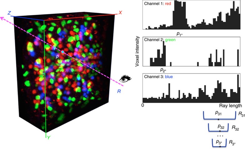
Three-dimensional (3D) bioimaging, visualization and data analysis are in strong need of powerful 3D exploration techniques. We develop virtual finger (VF) to generate 3D curves, points and regions-of-interest in the 3D space of a volumetric image with a single finger operation, such as a computer mouse stroke, or click or zoom from the 2D-projection plane of an image as visualized with a computer. VF provides efficient methods for acquisition, visualization and analysis of 3D images for roundworm, fruitfly, dragonfly, mouse, rat and human. Specifically, VF enables instant 3D optical zoom-in imaging, 3D free-form optical microsurgery, and 3D visualization and annotation of terabytes of whole-brain image volumes. VF also leads to orders of magnitude better efficiency of automated 3D reconstruction of neurons and similar biostructures over our previous systems. We use VF to generate from images of 1,107 Drosophila GAL4 lines a projectome of a Drosophila brain.

Figure 1. Curve drawing methods in the family of 3D VF algorithms.

CDA1 and CDA2 for generating a 3D curve using one computer-mouse stroke painted in the 2D projection of a 3D image of a dragonfly thoracic ganglion neuron. R₁~R_N: the first to the last shooting rays, which are parallel to each other and along the path of the mouse stroke. p₁~p_N: the estimated 3D location of each curve knot, each corresponding to a shooting ray. q_k,i and q_(k+1),i: the one-voxel evenly spaced 3D locations along the kth and (k+1)th rays, respectively; the final knot location p_k for the ray R_k is selected from the set.

Figure 2. Schematic illustration of several different methods of CDA.

Case 1: p₁ is determined using PPA, then search p₂ on the ray R₂ within a small range (the default was set to ±30 voxels in our software) around the location of p₁. Once p_k is found, the same method is reused to find p_k+1. This scheme is the CDA1 method, which is fast and useful for drawing in dark region, but is sensitive to the starting location. Case 2: Instead of determining p₁ using PPA, we directly use fast-marching to find the shortest Geodesic path between all possible points on the rays R₁ and R₂. The hit points will be called p₁ and p₂. Next, we find the shortest path between p₂ and the ray R₃, and thus find p₃. This process is repeated until all rays have been searched. This is the basic CDA2 method. Note, as all possible combination paths between R₁ and R₂ have been searched, this method is not sensitive to noise or obscuring of 3D objects (Supplementary Movies 6 and 7). Case 3: In CDA2, instead of finding the shortest path between one single hit point p_k on the ray R_k to the next ray R_k+1, we find the shortest paths for all consecutive rays. This then allows us to compute and choose the global minimum cost path starting from the first ray and ending at the last ray, in all possible combinations of initial paths through consecutive rays. The entire search area A1, that is, the whole overlapping area of rays and the 3D image, is used. This is called the globally optimal CDA2 method (Supplementary Movie 5). Case 4: We can first use PPA to determine preliminary hit points on a pair of consecutive rays, based on which a smaller search area A₂ is determined. A₂ consists of a series of margin-extended and tilted bounding boxes (default margin is 5 voxels). Next, we can restrict the search of CDA2 on A₂, instead of a much bigger region A₁. This scheme is called the bounding-box-restricted CDA2. Of note, for all above cases (and other additional cases explained in the Methods), we restrict the search to voxels only (instead of sub-voxel locations).

Figure 3. PPA_c for multiple colour-channel 3D pinpointing using one computer-mouse click.

Image shown: a confocal image of a Drosophila late embryo where cells are labelled using fluorophores with different colours. R: a shooting ray from the observer to the on-screen 2D mouse-click locus. p: the final 3D location estimated by finding the one with the maximal intensity among candidates p_1*, p_2* and p_3*, which are detected for all colour channels independently. For each colour channel, the progressive mean-shift method is used to narrow down the search range R_ik (in this case i=1, 2, 3, and the iteration indicator k=1, 2, …) along the shooting ray until convergence.

Figure 4. Evaluation of CDA.

(a) CDA generates consistent 3D neurite tracts (curves) (green and blue) that are very close to the ground truth (red) regardless of different viewing angles. Image: 3D confocal image of a heavy-noise-contaminated dragonfly thoracic ganglion neuron. The ‘ground–truth’ curves were generated using Vaa3D-Neuron1 (ref. 8) and were also manually inspected to ensure that they are correct. (b) Distances between the 3D neurite tracts (curves), which are generated from different angles and different zooms, and the ground truth. Data is based on 1,470 measurements of 7 tracts in the image in a. (c) Percentages of curve knots that have visible spatial difference (≥ 2 voxels) (mean±s.d.). 2D/2.5D: manual generation of a 3D curve based on first mouse-clicking on 2D cross-sectional XY planes in a 3D image, or using all three XY, YZ and ZX cross-sectional planes (2.5D), and then concatenating these locations sequentially. 3D PPA: manual generation of a 3D curve based on first mouse-clicking in the 3D-rendered image using PPA to produce a series of 3D locations, and then concatenating them. Data are based on tracing the primary projection tracts in five 3D dragonfly confocal images where the curve generation is possible for all the 2D/2.5D, 3D PPA and 3D CDA methods. (d) Speed of 3D curve generation using different methods (mean±s.d.). c-time, computing time for CDA; t-time, total time (including human-machine interaction and c-time) for CDA. Image data are the same in c.

Figure 5. Instant 3D zoom-in imaging and quantitative measurement of single-nucleus gene expression for C. elegans.

(a) A 3D pre-scan image of L1 C. elegans, along with the instant 3D measurements of gene expression levels of three cells BWMDL23, DEP and BWMDL24. p: location of interest for zoom-in imaging at a higher resolution. (b) Digital zoom-in of the area around p, where the insufficient voxel resolution does not manifest clear nuclei boundary. (c) Optical zoom-in around p, where the boundary between several nuclei is visible. (d) Instant 3D measurement of the gene expression of two bundles of body wall muscle cells, without computational segmentation of cells. For the profile of each curve of c₁ and c₂, the top is the gene expression of channel 1 (red) and bottom is that for channel 2 (green). Red: Punc54::H1::cherry. Green: Pmyo3::eGFP.

Figure 6. Instant 3D microsurgery for different animals.

(a) Instant 3D pinpointing of body wall muscle cells in a fixed L1 C. elegans worm. p₁, p₂, p₃: three muscle-cell nuclei. Red: Punc-54::H1::mCherry. Green: Pmyo-3::eGFP. (b) Instant 3D bleaching of the muscle cell nuclei in a. (c) Instant 3D pinpointing of muscle cells in a live L1 C. elegans worm. p₄, p₅: two muscle cells. Red: Pmyo-3::tagRFP-T. Green: Pmyo-3::GCaMP3. (d) Instant 3D bleaching of the muscle cells in c leads to bending of the animal. (e) Instant 3D pinpointing for an ato-GAL4-labelled Drosophila brain. p₆: a cell body of a neuron. p₇, p₈: two loci on a major ato-GAL4 neurite tract. Green: ato-GAL4 pattern. (f) Instant 3D bleaching of locations in e and instant 3D curving for the same specimen. c₁: a 3D curve cutting through the arbor of ato-GAL4 pattern in the optic lobe. (g) Instant 3D bleaching of the c₁ curve in f.

Figure 7. Instant 3D visualization of massive 3D image data stacks.

(a) Visualization of a 2.52-Tb whole-mouse brain image stack, which has 30,000 × 40,000 × 700 voxels and three 8-bit fluorescent channels. For each scale (S0~S4) when a user is using 3D VF’s one mouse stroke feature to zoom-in at arbitrarily defined 3D ROI, the ROI-computing time and the actual 3D rendering time for this ROI are also shown on top of each magenta arrow. (b) Bench-test of ROI-computing time (mean±s.d.) for five different large image stacks of different properties on different operating systems (Mac, Linux and Windows). The five images are: single mouse neuron (22.8 Gb, 16 bit, single channel, 11.4 Gigavoxels), two rat neurons (96.0 Gb, 8 bit, two channels, 48.0 Gigavoxels), hippocampus (330.3 Gb, 8 bit, single channel, 330.3 Gigavoxels), whole-mouse brain (504 Gb, 8 bit, 3 channels, 168 Gigavoxels) and another whole-mouse brain (2.52 Tb, 8 bit, 3 channels, 840 Gigavoxels). See Methods for the configurations of machines used in these tests. (c) The actual 3D rendering time to visualize the image contents in each computed ROI, bench tested for the same data sets in b and various operating systems.

Figure 8. Neuron reconstruction using Vaa3D-Neuron2.

(a) Reconstructions of a Drosophila projection neuron from a dark 3D confocal image. In the zoom-in region R, the image intensity is enhanced for better visibility. The two reconstructions are produced using two different tracing spans defined by two independent sets of landmark points. The reconstructions are intentionally offset from the image for comparison. e₁ and e₂: locations of small discrepancy of the two reconstructions. (b) Improvement of the reconstruction precision for ten Drosophila neurons, each with two independent trials of reconstructions. Manual reconstructions here were produced using Neurolucida. (c) Reconstruction of a densely arborized dragonfly thoracic neuron from a 3D confocal image with heavy noise. (d) Comparison of the computational complexity of competing methods for faithful reconstruction of 22 noise-contaminated dragonfly neurons.

Figure 9. A whole Drosophila-brain projectome of neuron tracts.

(a) Neuron tracts (9,198) extracted from 3D-registered confocal images of 1,107 GAL4 lines. The tracts that connect the same starting and ending brain compartments are colour matched. (b) The simplified projectome of neuronal patterns among different brain compartments. Scale bar, log₁₀ of the number of projections between compartments.

Figure 10. Vaa3D-Neuron2 reconstructions for other biological and biomedical applications.

(a,b) The 3D reconstructed bronchial tree of a mouse lung from two view angles. (c) The 3D reconstruction of a human brain angiogram. See refs , for exemplar details of the raw images and their biological applications for developmental biology, stem cell and human anatomy.

References

1. Walter T. et al.. Visualization of image data from cells to organisms. Nat. Methods 7, S26–S41 (2010). - PMC - PubMed
1. Eliceiri K. W. et al.. Biological imaging software tools. Nat. Methods 9, 697–710 (2012). - PMC - PubMed
1. Long F., Zhou J. & Peng H. Visualization and analysis of 3D microscopic images. PLoS Comput. Biol. 8, e1002519 (2012). - PMC - PubMed
1. Pologruto T. A., Sabatini B. L. & Svoboda K. ScanImage: flexible software for operating laser scanning microscopes. Biomed. Eng. Online 2, 13 (2003). - PMC - PubMed
1. Edelstein A., Amodaj N., Hoover K., Vale R. & Stuurman N. Computer control of microscopes using μManager. Curr. Protoc. Mol. Biol Chapter14, Unit14.20 (2010). - PMC - PubMed
Publication types
LinkOut - more resources