Quantitative susceptibility mapping (QSM): Decoding MRI data for a tissue magnetic biomarker

Abstract

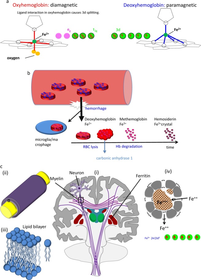
In MRI, the main magnetic field polarizes the electron cloud of a molecule, generating a chemical shift for observer protons within the molecule and a magnetic susceptibility inhomogeneity field for observer protons outside the molecule. The number of water protons surrounding a molecule for detecting its magnetic susceptibility is vastly greater than the number of protons within the molecule for detecting its chemical shift. However, the study of tissue magnetic susceptibility has been hindered by poor molecular specificities of hitherto used methods based on MRI signal phase and T2* contrast, which depend convolutedly on surrounding susceptibility sources. Deconvolution of the MRI signal phase can determine tissue susceptibility but is challenged by the lack of MRI signal in the background and by the zeroes in the dipole kernel. Recently, physically meaningful regularizations, including the Bayesian approach, have been developed to enable accurate quantitative susceptibility mapping (QSM) for studying iron distribution, metabolic oxygen consumption, blood degradation, calcification, demyelination, and other pathophysiological susceptibility changes, as well as contrast agent biodistribution in MRI. This paper attempts to summarize the basic physical concepts and essential algorithmic steps in QSM, to describe clinical and technical issues under active development, and to provide references, codes, and testing data for readers interested in QSM.

Keywords: Bayesian; QSM; calcification; contrast agent; dipole field; dipole kernel; ferritin; gradient echo; hemoglobin; hemorrhage; iron; metabolism; morphology enabled dipole inversion; myelin; oxygen consumption; quantification; quantitative susceptibility mapping.

Figure 1

Biomedical magnetic materials. (a) Diamagnetic hemoglobin and paramagnetic deoxyhemoglobin. During metabolic consumption of oxygen in the brain, heart, and kidney, weakly diamagnetic oxyhemoglobin releases O₂ and becomes strongly paramagnetic deoxyhemoglobin. Whereas the 3d electron orbits of Fe²⁺ in deoxyhemoglobin may be approximated as an isolated iron atom with four unpaired electrons (right), the intramolecular interaction between the porphyrin ring and Fe²⁺ in oxyhemoglobin (ligand interaction) splits the Fe atom’s 3d-orbit into two levels, e_g and t_2g, with all six electrons paired in the three t_2g orbits. (b) Blood degradation in hemorrhage. Following the onset of a hemorrhage, a small fraction of red blood cells (RBCs) may be endocytosed by microglia/macrophages. The majority of RBCs undergo cell lysis and hemoglobin (Hb) degradation from deoxyhemoglobin into methemoglobin (Fe³⁺) and hemosiderin (possible magnetic domain). Modeled after: Lancet Neurol 2012;11:720–731. (c) Susceptibility sources in the human brain. Major susceptibility sources in (i) the brain include myelin and ferritin. The white matter tracts in the brain consist of myelinated nerve fibers. (ii) Zoomed view of the box in (i) showing axon (yellow) and myelin sheath (purple). Myelin consists of several layers of lipid bilayer. (iii) Zoomed view of the box in (ii) showing a lipid bilayer and an individual lipid. (iv) Ferritin in a cross-section. Ferritin consists of a peptide spherical shell 2-nm thick with a 8-nm diameter cavity. Fe²⁺ enters through a four-fold symmetric channel, is stored as Fe³⁺ oxide mineral, and is released as Fe²⁺ through a three-fold symmetric channel. There are five unpaired 3d electrons in Fe³⁺, generating strong paramagnetism.

Figure 2

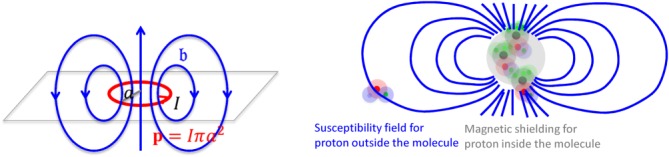
Magnetic fields, chemical shift, and magnetic susceptibility.(Left) The field of a magnetic dipole modeled by a current loop of radius. At the loop center, as.(Right) The electron cloud of a molecule polarized by generates magnetic shielding or chemical shift for the observer proton in the molecule and a susceptibility field (in dipole pattern) for the observer proton outside the molecule.

Figure 3

Schematics for quantitative susceptibility mapping. Quantitative susceptibility mapping (QSM) in general consists of three steps. Step 0: Generate magnitude image and field with unwrapping. Step 1: Remove background field and generate tissue field. Step 2: Generate QSM from tissue field and magnitude image.

Figure 4

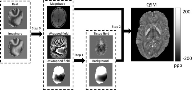
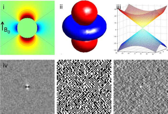
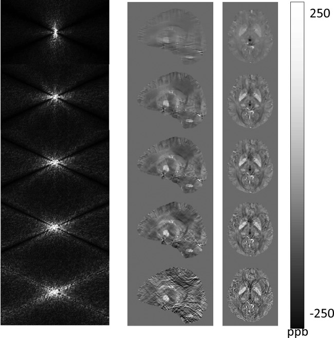
The ill-posedness of the dipole inverse problem. The unit dipole field in sagittal section (i) and its surface rendered contour (ii). (iii) The zero cone surfaces of the dipole kernel in k-space. (iv) Field map derived at signal-to-noise ratio (SNR) – 20 induced by a point source. (v, vi) Susceptibility in image space obtained by truncated k-space division with the threshold – 0 and 0.1. As a consequence of the dipole kernel zero behavior in the cone surface neighborhood, there is substantial noise propagation from the field measurements into the susceptibility estimate (40), as illustrated in an example of reconstruction by direct division (v and vi). A little noise added in the phase map (peak SNR – 20) leads to a totally corrupted susceptibility image that bears no physical resemblance to the true susceptibility source.

Figure 5

Background field removal using various algorithms. The tissue fields in a healthy volunteer estimated using HPF, LBV, SHARP, RESHARP, and PDF methods, respectively, demonstrate similar tissue patterns but with slight and different accents. HPF, high-pass filtering; LBV, Laplacian boundary value; PDF, projection onto dipole fields; RESHARP, regularization enabled SHARP; SHARP, sophisticated harmonic artifact reduction on phase data.

Figure 6

Evolution of susceptibility solutions in conjugate gradient. Susceptibility images in k-space (left column) and r-space after the first, third, fifth, 10th, and 100th iterations using the conjugate gradient solver demonstrate that the none-cone region in k-space converges quickly in the first few iterations; and the later iterations mainly contribute to signal in the cone region that manifests as streaking artifacts in the sagittal view and noise in the axial view in r-space.

Figure 7

Comparison of various quantitative susceptibility mapping reconstruction methods. QSM images are reconstructed using various methods from left to right and then top to bottom: TSVD, TKD, iSWIM, CSC, COSMOS, MEDI, HEIDI, TVSB, and R2* map. Most similar to COSMOS are MEDI, CSC, and HEIDI, with only very subtle differences among them: CSC has less black dots; MEDI has better defined dorsomedial nuclei of thalamus. CSC, compressed sensing compensated; COSMOS, calculation of susceptibility using multiple orientation sampling; HEIDI, homogeneity-enabled incremental dipole inversion; MEDI, morphology-enabled dipole inversion; QSM, quantitative susceptibility mapping; TKD, truncated-space division; TSVD, truncated singular value decomposition; TVSB, total variation using split Bregman.

Figure 8

Quantitative susceptibility mapping for measuring diamagnetic biomaterials such as calcifications. Top row: susceptibility of calcification measured on QSM (dark oval in right thalamus) demonstrates very good linear correlation with Hounsfield units measured on CT. Twenty six patients (64 calcifications) were included in the linear regression. Bottom row: Neurocysticercosis in T2* weighted, magnitude, phase, SWI, QSM, and CT images has both calcified and active lesions. Among all MRI images, only QSM shows the active lesion with positive susceptibility (red arrow) and clearly show the calcified lesions with negative susceptibilities (yellow arrows). The CT section is slightly tilted from the orientation of the MRI section, causing a discrepancy in the lesion’s appearances. QSM, quantitative susceptibility mapping; SWI, susceptibility weighted imaging. Source: Chen et al, Radiology 2014;270:496–505.

Figure 9

Quantitative susceptibility mapping for measuring paramagnetic heme iron. The total susceptibility of a cerebral microbleed measured on QSM is a physical property that is independent of TE, providing a universal measure for cerebral microbleeds burden (10 patients with 40 microbleeds). Left image panel: Microbleed appearance changes with TE (15 msec top row; 46 msec bottom row) drastically in magnitude and moderately in the R2* map but little in QSM (white arrows). Ventricle calcifications have the same sign on T2*w and R2* but opposite sign on QSM (black arrows) as microbleeds. Right graph: When TE was increased from approximately 20 to 40 msec, the measured cerebral microbleed volume increased by mean factors of 1.49 ± 0.86 (standard deviation), 1.64 ± 0.84, and 2.30 ± 1.20, respectively, for QSM, R2*, and T2*w, respectively (P < .01). However, the measured total susceptibility with QSM did not show significant change over TE (P – .31), and the variation was significantly smaller than any of the volume increases (P < .01 for each). QSM, quantitative susceptibility mapping; TE, echo time. Source: Liu et al, Radiology 2012;262:269–278.

Figure 10

Quantitative susceptibility mapping for visualizing deep brain stimulation targets. Globus pallidus interna (GPi) and subthalamic nucleus (STN), surgical targets for deep brain stimulation, are either invisible or inseparable from surrounding tissues on T2W image (with zoom), but are clearly visualized on deep brain stimulation (QSM) (with zoom). Other basal ganglia structures well-defined on QSM include globus pallidus pars externa (GPe) and substantia nigra (SN). Source: Liu et al, Radiology 2013;269:216–23.

Figure 11

Quantitative susceptibility mapping for quantifying paramagnetic contrast agents. In an in vivo dynamic gadolinium (Gd) enhancement study of the brain, time-resolved Quantitative susceptibility mapping (QSM) was developed using spiral readout and temporal resolution acceleration with constrained evolution reconstruction (TRACER) complex image reconstruction. The difference image divided Gd molar susceptibility generates time-resolved Gd concentration map. Source: Xu et al, MRM 2014, epub.

Figure 12

Quantitative susceptibility mapping for quantifying a mixture of paramagnetic and diamagnetic biomaterials. (i) Acute enhancing lesions in a 32-year-old male with RRMS at two time points: initial study (T1w + c1 and QSM1, 1st row) and 3-month follow-up (T1w + c2 and QSM2, 2nd row) (T1w + c – T1-weighted imaging with Gd). Lesions appear in the right frontal WM (white arrows) and in the lcc (black arrows). Both lesions are enhancing (arrows) on T1w + c1 and isointense (white boxes) on QSM1. The lesions changed on follow up to nonenhancing on T1w + c2 and hyperintense on QSM2 (arrows). The right frontal WM matter lesion shrunk between QSM1 and QSM2. The lcc lesion (black arrow) recovered to normal appearing on T2w and T1w (not shown), T1w + c. (ii) Nonenhancing lesions (33y, f, RRMS) on QSM at two time points (2nd row was 6 months later). All QSM lesions at time point 1 were estimated to be 1.2y using prior MRIs. All lesions (arrows) are QSM hyperintense on both time points with similar values. (iii) Chronic nonenhancing lesions (50y f RRMS) on QSM and T2W. Two lesions over 10 years old were detected (white arrows). They appear isointense on both QSM (white boxes, only initial study shown). lcc, left cingulate cortex; QSM, quantitative susceptibility mapping; RRMS, relapsing-remitting multiple sclerosis; WM, white matter. Source: Chen et al, Radiology 2014;271:183–192.

Figure 13

Time course of susceptibilities of multiple sclerosis lesions. The susceptibility time course may provide new insight into pathophysiologic features of MS lesions (23 patients with 162 lesions): Magnetic susceptibility of MS lesion increases rapidly as it changes from enhanced to nonenhanced, attains a high-susceptibility value relative to NAWM during its initial few years (approximately 4 years), and gradually dissipates back to susceptibility similar to that of NAWM as it ages. The graphs depict lesion susceptibility values (relative to NAWM) at various ages in QSM1 performed at a first time point (top) and in QSM2 at a second time point (bottom). Red points in QSM1 denote acute enhancing lesions at lesion age – 0 year; follow-up presented as green points in QSM2 demonstrated a substantial increase in susceptibility. Blue lines represent average susceptibilities of nonenhanced lesions in the age groups of 0 to 2, 2 to 4, 6 to 8, and 8 to 10 years and enhancing lesions. QSM, quantitative susceptibility mapping; MS, relapsing-remitting multiple sclerosis; NAWM, normal appearing white matter. Source: Chen et al, Radiology 2014;271:183–192.

Figure 14

Quantitative susceptibility mapping applications in the breast and liver. (i) Left image is a mammogram and right image is the corresponding QSM (minimal intensity project through the 3D volume) of a breast in a female patient with three calcified nodules (arrow on QSM). Fatty tissues in the breast appear less diamagnetic compared to the gland. (ii) QSM and R2* images of a liver are shown in the left and right, respectively. Hepatic vein and subcutaneous fat (white arrows in left) appear paramagnetic. The susceptibility difference between the hepatic vein (white arrow) and the aortic artery (black arrow) are 0.53 ppm. 3D, three dimensional; QSM, quantitative susceptibility mapping.

References

1. Wang Y. 2012. . Principles of Magnetic Resonance Imaging: physics concepts, pulse sequences & biomedical applications. Available at: www.createspace.com/4001776. Accessed December 1, 2013.
1. de Crespigny AJ, Roberts TP, Kucharcyzk J, Moseley ME. Improved sensitivity to magnetic susceptibility contrast. Magn Reson Med. 1993;30:135–137. - PubMed
1. Haacke EM, Xu Y, Cheng YC, Reichenbach JR. Susceptibility weighted imaging (SWI) Magn Reson Med. 2004;52:612–618. - PubMed
1. Haacke EM, Reichenbach J. Susceptibility weighted imaging in MRI: basic concepts and clinical applications. Hoboken, NJ: Wiley-Blackwell; 2011.
1. Jackson JD. Classical electrodynamics. 3rd ed. Hoboken, NJ: John Wiley and Son; 1999. pp. 184–188.
Publication types