Learning Instance-Specific Predictive Models

Abstract

This paper introduces a Bayesian algorithm for constructing predictive models from data that are optimized to predict a target variable well for a particular instance. This algorithm learns Markov blanket models, carries out Bayesian model averaging over a set of models to predict a target variable of the instance at hand, and employs an instance-specific heuristic to locate a set of suitable models to average over. We call this method the instance-specific Markov blanket (ISMB) algorithm. The ISMB algorithm was evaluated on 21 UCI data sets using five different performance measures and its performance was compared to that of several commonly used predictive algorithms, including nave Bayes, C4.5 decision tree, logistic regression, neural networks, k-Nearest Neighbor, Lazy Bayesian Rules, and AdaBoost. Over all the data sets, the ISMB algorithm performed better on average on all performance measures against all the comparison algorithms.

Keywords: Bayesian model averaging; Bayesian network; Markov blanket; instance-specific.

Figure 1

A general characterization of the induction of and inference in population-wide (top panel) and instance-specific (bottom panel) models. In the bottom panel, there is an extra arc from instance to model, because the structure and parameters of the model are influenced by the features of the instance at hand.

Figure 2

A simple hypothetical Bayesian network for a medical domain. All the nodes represent binary variables, taking values in the domain T, F where T stands for True and F for False. The graph at the top represents the Bayesian network structure. Associated with each variable (node) is a conditional probability table representing the probability of each variable’s value conditioned on its parent set. (Note: these probabilities are for illustration only; they are not intended to reflect frequency of events in any actual patient population.)

Figure 3

Example of a Markov blanket. The Markov blanket of the node X₆ (shown stippled) comprises the set of parents, children and spouses of the node and is indicated by the shaded nodes. The nodes in the Markov blanket include X₂ and X₃ as parents, X₈ and X₉ as children, and X₅ and X₇ as spouses of X₆. X₁, X₄, X₁₀ and X₁₁ are not in the Markov blanket of X₆.

Figure 4

Constraints on the Markov blanket operators. The nodes are categorized into five groups: T = target, P = parent, C = child, S = spouse, and O = other (not in the Markov blanket of T). The cells with check marks indicate valid operations and are the only ones that need to be considered in generating candidate structures. The cells with an asterisk indicate that the operation is valid only if the resulting graph is acyclic.

Figure 5

An example where the application of an operator leads to additional removal of arcs to produce a valid Markov blanket structure. Deletion of arc Z → X₅ leads to removal of the arc X₄ → X₅ since X₅ is no longer a part of the Markov blanket of Z. Reversal of the same arc also leads to removal of the arc X₄ → X₅ since X₅ is now a parent and is precluded from having incoming arcs. Also, unless X₄ → X₅ is removed there will be a cycle.

Figure 6

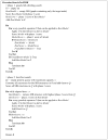
Pseudocode for the two-phase search procedure used by the ISMB algorithm. Phase 1 uses greedy hill-climbing search while phase 2 uses best-first search.

Figure 7

Training and test data sets derived from the deterministic function Z = A ∨ (B ∧ C ∧ D). The training set contains a total of 69 instances and the test set a total of three instances as shown; the test instances are not present in the training set. The training set simulates low prevalence of A = T since only five of the 69 instances have this variable-value combination.

Figure 8

Plots of model averaged estimate of P(Z^t = T|x^t,D) that is abbreviated as P(Z = T) and model score obtained by ISMB and NISMB algorithms on the three test cases given in Figure 7. Each row represents a single test case with the plot on the left obtained from the ISMB algorithm and the plot on the right obtained from the NISMB algorithm. The value of the final averaged estimate of P(Z^t = T|x^t,D) is the point where the darker curve meets the Y-axis on the right.

References

1. Aha DW. Feature weighting for lazy learning algorithms. In: Huan L, Hiroshi M, editors. Feature Extraction, Construction and Selection: A Data Mining Perspective. Kluwer Academic Publisher; Norwell, MA: 1998. pp. 13–32.
1. Aliferis CF, Tsamardinos I, Statnikov A. Hiton: A novel markov blanket algorithm for optimal variable selection. Proceedings of the American Medical Informatics Association (AMIA) Annual Symposium; 2003. pp. 21–5. - PMC - PubMed
1. Aliferis CF, Statnikov A, Tsamardinos I, Mani S, Koutsoukos XD. Local causal and markov blanket induction for causal discovery and feature selection for classification part i: Algorithms and empirical evaluation. Journal of Machine Learning Research. 2010a Jan;11:171–234.
1. Aliferis CF, Statnikov A, Tsamardinos I, Mani S, Koutsoukos XD. Local causal and markov blanket induction for causal discovery and feature selection for classification part ii: Analysis and extensions. Journal of Machine Learning Research. 2010b Jan;11:235–284.
1. Atkeson CG, Moore AW, Schaal S. Locally weighted learning. Artificial Intelligence Review. 1997;11(1–5):11–73.
LinkOut - more resources