Selective responses to tonic descending commands by temporal summation in a spinal motor pool

Abstract

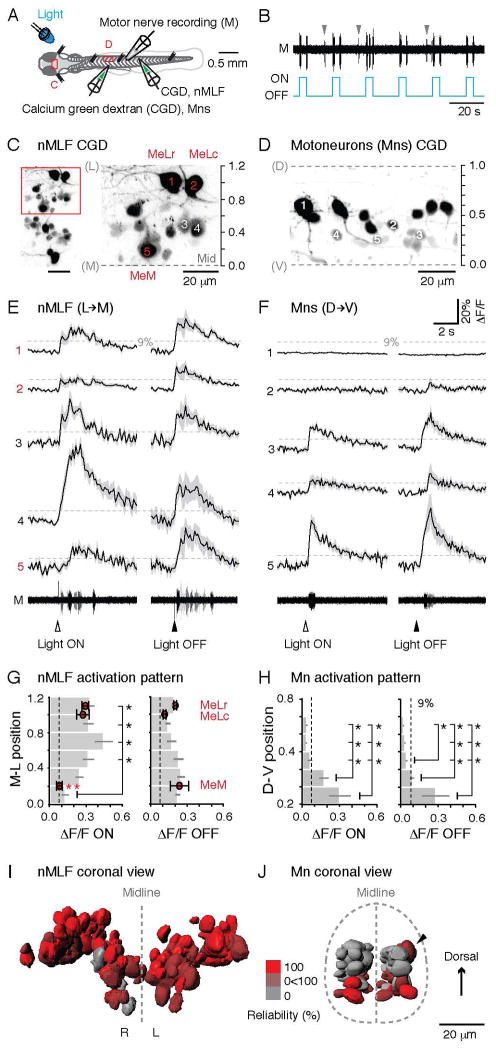
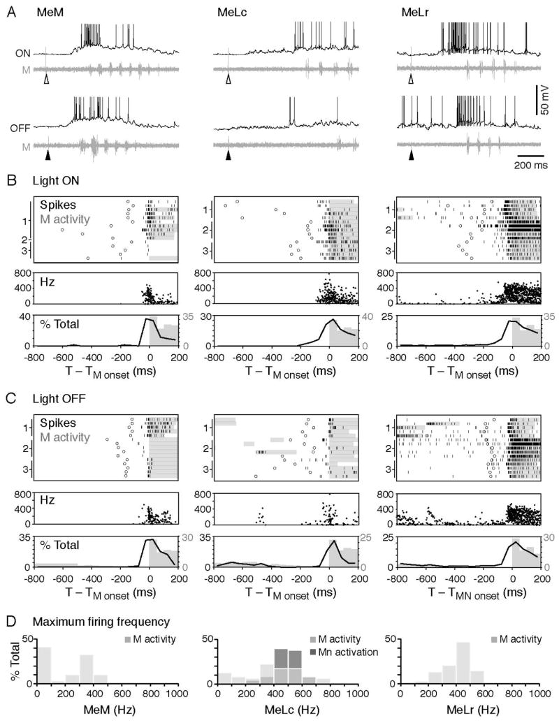
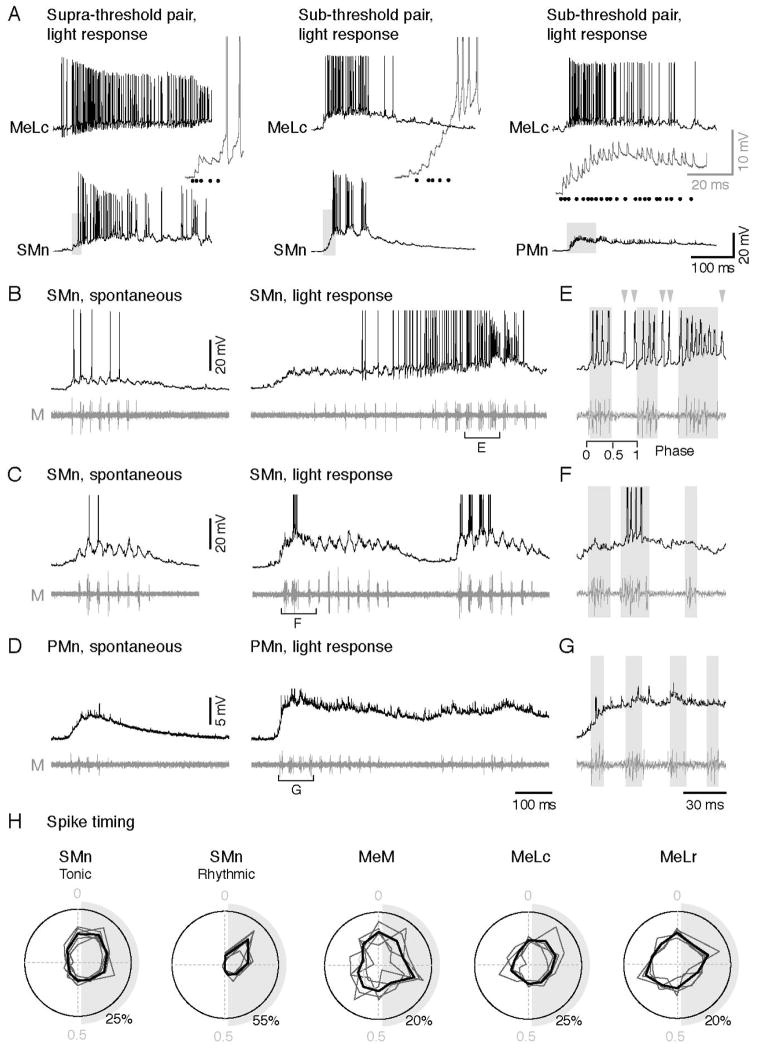
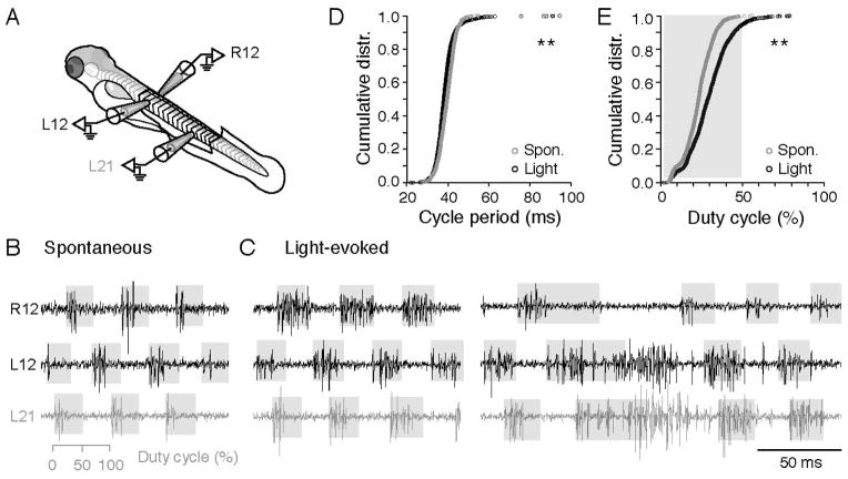
Motor responses of varying intensities rely on descending commands to heterogeneous pools of motoneurons. In vertebrates, numerous sources of descending excitatory input provide systematically more drive to progressively less excitable spinal motoneurons. While this presumably facilitates simultaneous activation of motor pools, it is unclear how selective patterns of recruitment could emerge from inputs weighted this way. Here, using in vivo electrophysiological and imaging approaches in larval zebrafish, we find that, despite weighted excitation, more excitable motoneurons are preferentially activated by a midbrain reticulospinal nucleus by virtue of longer membrane time constants that facilitate temporal summation of tonic drive. We confirm the utility of this phenomenon by assessing the activity of the midbrain and motoneuron populations during a light-driven behavior. Our findings demonstrate that weighted descending commands can generate selective motor responses by exploiting systematic differences in the biophysical properties of target motoneurons and their relative sensitivity to tonic input.

Figure 1. Differences in the Dorso-ventral Distribution of Spinal Axon Collaterals among the Identified nMLF Neurons

(A) A schematic of a larval zebrafish viewed from above (A1). The brain area is expanded in A2 to show the retrogradely labeled descending neurons in the midbrain and hindbrain. The red box highlights the nMLF (nucleus of the medial longitudinal fasciculus). In A3, the three large, identified nMLF neurons are marked. Mid = midline. Scale bar = 20 μm. (B, C) Top-down view of the retrogradely labeled nMLF (white), with two identified nMLF neurons labeled with different colored dyes in the same fish (red and green). (D) A schematic of a larval zebrafish viewed from the side (D1). Lateral view of the reconstructed main axon and collaterals of a MeM (D2), MeLc (D3), and MeLr (D4) neuron in the spinal cord from the region indicated in red on the schematic. (E, F) Lateral view of the spinal cord with the main axon and collaterals of two identified nMLF neurons labeled with different colored dyes in the same fish. Cells are the same as those presented in B and C. White tick marks divide the dorso-ventral extent of spinal cord into 10 equal divisions. (G) Total collateral length from body segments 5–14 at each dorso-ventral division for the MeLr and MeM neurons shown in B and E, normalized to the top (1) and bottom (0) edges of spinal cord. (H) As in G, but for the MeLr and MeLc neurons shown in C and F. (I) Contribution of MeM, MeLc, and MeLr neurons to the total amount of their spinal collaterals expressed as a percentage. Analysis was restricted to the dorso-ventral divisions 0.2–0.7, where spinal motoneurons are located (n = 5 for each cell type). The MeM neuron contributes more to the total collateral length at division 0.2 (black arrowhead), due to its ventral commissural collaterals.

Figure 2. Identified nMLF Neurons Connect to Spinal Motoneurons

(A) Images of the spinal cord of a parg^mn2ET zebrafish larva, in which GFP is expressed in spinal motoneurons, from the side (A1) and in cross-section (A2). In A1, the four large, dorsally-located primary motoneurons (PMns) in one body segment are marked by red arrowheads. In A2, the schematic on the right half demarcates the locations of motoneuron cell bodies and neuropil. Dashed lines indicate the boundary of spinal cord and midline. (B–D) Confocal Z-stacks of spinal axon collaterals of nMLF neurons (in red) and axial motoneurons (in white) in parg^mn2Et zebrafish larvae. Images are from the side (B1–D1) and in cross section (B2–D2). The depth of the Z-stacks is ~20 μm in B1–D1. The cross-sectional images in B2–D2 represent a collapsed view from one body segment (~80–90 μm). (E) Coronal view of reconstructed axon collaterals from MeM, MeLc, and MeLr neurons registered to anatomical landmarks (n = 4 for each cell type), with the cell body and neuropil layers marked as in A2. IL, ipsilateral; CL, contralateral. (F) Schematic showing the preparation for paired-whole cell patch clamp recordings from nMLF neurons and spinal motoneurons. (G–I) Example traces from paired recordings from the MeM (G), MeLc (H) and MeLr (I) and a PMn. Individual evoked EPSPs from each pair (gray lines, n = 10 per pair) and an averaged waveform (black line) are temporally aligned to the peak of nMLF action potentials (red, averaged waveform). (J) Peak amplitude of the early and later components of evoked EPSPs in the PMns. Double asterisks indicate significance (Mann-Whitney U-test with Bonferroni corrections for multiple comparisons, p<0.05). n/s = not significant. Here and elsewhere, data are reported as mean +/− SEM.

Figure 3. Differences in the Waveforms of MeLc-Evoked EPSPs Related to Motoneuron Input Resistance

(A) Example of direct connections between the MeLc neuron and a larger, dorsal PMn (see schematic in upper right corner) in control solution, high-divalent cation solution (Ca²⁺/Mg²⁺), or in the presence of the glutamate receptor antagonists NBQX/AP5. Superimposed EPSPs (gray lines, n = 10) and their averaged trace (black line) are shown in each example. (B) As in A, but direct connections between a MeLc neuron and a smaller, ventral SMn. Note, in this example the control panels and spikes are the same because the hi-divalent and NBQX/AP5 perfusions were performed in the same fish (*). (C) Comparison of MeLc-evoked EPSPs that contain only the early, electrical component in PMns and SMns. Standard error is indicated by the shading. EPSP waveforms have been scaled and aligned to peaks to illustrate the slower decay in the SMns compared to the PMns. (D) As in C, but for EPSPs that contain a clear chemical component in PMns and SMns. (E) Properties of MeLc-elicited EPSPs that contain only the early component versus input resistance (Rin) of spinal motoneurons. These include EPSP amplitude (E1), rise time (E2), half-width (E3), and decay time constant (E4). Trend line is a linear fit. **: p<0.05 following Spearman’s rank test (ρ). (F) Reliability of the later, chemical component of MeLc-elicited EPSPs in PMns and SMns (PMn, 38 ± 7%, n = 8; SMn, 7 ± 2%, n = 11; Student’s t-test, **p<0.05) (G) As in E, but for EPSP amplitude (G1), half-width (G2) and decay time constant (G3) with clear chemical components.

Figure 4. Temporal Summation Enables Higher Rin Motoneurons to Fire

(A) Steps of increasing current levels (I) from left to right lead to increases in instantaneous spike frequency in the MeLc (left, 50 Hz; middle, 255 Hz; right, 480 Hz). MeLc action potentials elicit reliable EPSPs in the connected PMn (Rin = 56 MΩ), which never fires action potentials. (B) As in A, but for a more excitable SMn (Rin = 404 MΩ). Increases in the instantaneous spike frequency of the MeLc (left, 75 Hz; middle, 260 Hz; right, 480 Hz) are sufficient to get the SMn to fire action potentials. (C) Expanded view of EPSPs evoked by the first two spikes in the current step from the gray (low MeLc firing frequency) and red (high frequency) shaded areas in A. The gray line connects the peaks of the first two EPSPs (arrowheads) and the resulting slope (ΔV) was used to calculate EPSP summation at different MeLc firing frequencies. Here, and elsewhere black dots mark the timing of corresponding MeLc action potentials. C and D share the same scale bars. (D) As in C, but for the SMn illustrated in B. Note the much larger ΔV in the top red trace compared to the PMn in C at the same MeLc firing frequency. The action potential is truncated (*). (E) The slope (ΔV) of the first two MeLc elicited EPSPs versus the firing frequency of the corresponding MeLc action potentials for the PMn and SMn shown in A–D. The slope of the linearly fit trend lines was used as the gain for EPSP summation for each motoneuron (PMn, R = 0.1; SMn, R = 0.92). (F) Gain of EPSP summation (the slope of the ΔV trend line as shown in E) versus EPSP decay time constant. **: p<0.05 following Pearson linear correlation test (R). (G) Rin versus membrane time constant of spinal motoneurons. The repolarization of the membrane potential (V) after a brief hyperpolarizing current (I) pulse (open red arrowhead) was fit with a single exponential equation to calculate the membrane time constant. Trend line is a linear fit. **: p<0.05 following Spearman’s rank test (ρ).

Figure 5. nMLF Neurons Reliably Respond to Changes in Illumination

(A) Schematic showing the preparation for calcium imaging of the nMLF neurons (C) or spinal motoneurons (D) using calcium green dextran (CGD) injections, and a simultaneous motor nerve (M) recording. LED, light emitting diode. (B) The onset/offset of the LED reliably elicits ‘fictive’ motor output, which can be recorded from the motor nerve in α-bungarotoxin immobilized preparations. Spontaneous motor output is marked by gray arrowheads. (C) View of the nMLF neurons backfilled with CGD from above (left), with a higher magnification of the area boxed in red (right). The midline (Mid) of the brain and the center of the MeLr soma were used as references for normalizing the medio-lateral (M-L) locations of nMLF neurons (midline = 0, MeLr soma = 1). (D) A subset of spinal motoneurons backfilled with CGD. Retrograde filling reliably labels motoneurons throughout the full dorso-ventral (D-V) range of the spinal motor column. Dashed lines mark dorsal (D) and ventral (V) boundaries of the spinal cord, normalized as 1 and 0. (E) Calcium transients associated with motor output for nMLF neurons at different M-L locations (marked in C) in response to light onset and offset (black line = averaged response; shaded area = standard error; n = 5 trials for each neuron). The dashed line marks 9% ΔF/F, the threshold for determining whether a neuron is active. For both E and F, arrowheads indicate time of the light stimuli. Motor nerve activity (M) for each of the five trials is superimposed in different shades of gray. E and F share the same scale bars. (F) Example calcium transients for motoneurons at different D-V locations (marked in D) in response to light onset and offset. The dashed line marks 9% ΔF/F. (G) Averaged calcium response amplitudes of nMLF neurons at different M-L locations in the midbrain. Light ON, n = 91 cells; light OFF, n = 52 cells; both from 8 fish. *: p<0.05 following Mann-Whitney U test and Bonferroni correction for multiple comparisons. Response amplitude of the three identified nMLF neurons are shown as red circles at their relative M-L locations. Light ON, n = 25 cells; light OFF, n = 18 cells; both from 8 fish. *: p<0.05 following Mann-Whitney U-test and Bonferroni correction for multiple comparisons. In G and H, dashed line marks the 9% ΔF/F. (H) Calcium response amplitude to light onset and offset of spinal motoneurons at different D-V locations in the spinal cord. Light ON, n = 127 cells from 11 fish; light OFF, n = 78 cells from 7 fish. *: p<0.05 following Mann-Whitney U test and Bonferroni correction for multiple comparisons. (I) 3D-registration of soma surfaces of nMLF neurons from 8 fish. The neuron surfaces are color-coded according to their reliability of response to light (100%, bright red, always responds to light; 0%, gray, never responds to light). Light onset and offset responses are pooled. R, right side; L, left side. (J) 3D-registration of soma surfaces of spinal motoneurons from 8 fish. The motoneuron surfaces are color-coded according to their reliability of response to light as described in J. A black arrowhead marks a more dorsal motoneuron that responded on the upper side of the side-lying fish.

Figure 6. High Frequency Firing of nMLF Neurons Precedes the Motor Response to Changes in Illumination

(A) Example traces of whole-cell recordings on the MeM (left), MeLc (middle), and MeLr (right) neurons together with motor nerve activity in response to light onset (at open arrowheads) and offset (at filled arrowheads). The action potentials of the MeLc and MeLr neurons are truncated. (B) Upper: raster plots demonstrate the firing pattern of the nMLF neurons in response to light onset (n = 15 trials from 3 neurons in each class, marked on the left of the raster plot). Firing is aligned to the start of the first swim bout (motor nerve activity) after the light stimulus (black ticks: nMLF action potential, circles: visual stimulus, gray bars: swim bout). Middle: Instantaneous firing frequency of nMLF action potentials shown in the raster plot. Lower: a histogram illustrates the distribution of nMLF action potentials (black line) and motor nerve swim bursts (gray bars). MeM, n = 16 trials from 4 neurons; MeLc, n = 31 trials from 5 neurons; MeLr, n = 34 trials from 5 neurons. (C) Response to the light offset. Figures are arranged as in B. MeM, n = 40 trials from 5 neurons; MeLc, n = 32 trials from 5 neurons; MeLr, n = 33 trials from 5 neurons. (D) Maximum spike frequency during light evoked swim bouts (M activity; MeM, 58 trials from 5 neurons; MeLc, 63 trials from 5 neurons; MeLr, 68 trials from 7 neurons). The MeLc spike frequencies that successfully activated motoneurons during current injection (Mn activity, illustrated in 4B, D) fall within the natural spike frequency range of MeLc neurons during swimming. The MeM neuron has more events at the 0–100 Hz frequency bin because in more trials the cell only fires a single action potential in response to light.

Figure 7. Increased Firing of SMns are Related to Tonic Activity in the nMLF during Light-evoked swimming

(A) Paired-whole cell recordings on the MeLc neuron and spinal motoneurons with different responses to MeLc current injection and light stimulus. Activity shown here is elicited by light. Left: a SMn that can be activated by firing the MeLc alone with current injection (supra-threshold pair). Middle: a SMn that cannot be activated by firing the MeLc alone (sub-threshold pair). Right: a PMn that cannot be activated by firing the MeLc alone. Insets are expanded view from the gray shading areas. MeLc spikes are represented as black dots. (B–D) Whole-cell recording of SMns (B–C) and a PMn (D) with a motor nerve recording during spontaneous and light evoked swimming. (E–G) Expanded view from the bracketed areas in B–D respectively to show phase relationship of action potentials and swimming bursts. Swim bursts are marked by gray shadings to highlight ‘in-phase firing’, while gray arrowheads mark ‘anti-phase’ firing. The phase of a swim cycle (0: start,1: end) is marked in E. (H) Polar plots show the phase relationship of action potentials to cyclical swim bursts during light response normalized to the start (0) and end (1) of the swim cycle (example shown in E). Gray shading represents half of the swim cycle. Spike phase distribution of individual cell (dark gray line) and the averaged distribution (black line) are shown. SMns are segregated into groups according to whether their firing pattern was tonic (n= 2,598 spikes from 6 neurons) or rhythmic (n = 435 spikes from 5 neurons). Action potentials of the MeM, MeLc, and MeLr neurons occur throughout the swim cycle consistent with tonic firing behavior (MeM, n = 803 spikes from 5 neurons; MeLc, n = 984 spikes from 4 neurons; MeLr, n = 1071 spikes from 4 neurons).

Figure 8. Light-Evoked Behavioral Responses are Primarily Characterized by Increases in the Durations of Alternating Motor Bursts

(A) Schematic of the preparation for recording motor nerves on the left (L) and right (R) sides of the body. (B) Spontaneous fictive motor bursts recorded at the 12^th body segment on the left and right sides, and the 21^st body segment on the left side. Shaded gray boxes indicate the 50% duty cycle on a burst-by-burst basis. During spontaneous swimming, motor bursts rarely exceed 50%. (C) As in B, but for light-evoked activity. Fictive swimming in response to light routinely reaches and can exceed a phase value of 0.5. (D) Cumulative distribution of cycle periods (time between successive motor bursts) for spontaneous and light-evoked motor activity. **: p<0.05, Kolmogorov-Smirnov test. (E) Cumulative distribution of the percentage of the swim cycle motor bursts occupy for spontaneous and light-evoked motor activity. **: p<0.05, Kolmogorov-Smirnov test.

References

1. Alstermark B, Isa T. Circuits for skilled reaching and grasping. Annu Rev Neurosci. 2012;35:559–578. - PubMed
1. Ampatzis K, Song J, Ausborn J, El Manira A. Pattern of innervation and recruitment of different classes of motoneurons in adult zebrafish. J Neurosci. 2013;33:10875–10886. - PMC - PubMed
1. Balciunas D, Davidson AE, Sivasubbu S, Hermanson SB, Welle Z, Ekker SC. Enhancer trapping in zebrafish using the Sleeping Beauty transposon. BMC Genomics. 2004;5:62. - PMC - PubMed
1. Bhatt DH, McLean DL, Hale ME, Fetcho JR. Grading movement strength by changes in firing intensity versus recruitment of spinal interneurons. Neuron. 2007;53:91–102. - PubMed
1. Bhatt DH, Otto SJ, Depoister B, Fetcho JR. Cyclic AMP-induced repair of zebrafish spinal circuits. Science. 2004;305:254–258. - PubMed
Publication types
LinkOut - more resources