

The importance of phenotypic data analysis for genomic prediction - a case study comparing different spatial models in rye
- PMID: 25087599
- PMCID: PMC4133075
- DOI: 10.1186/1471-2164-15-646
The importance of phenotypic data analysis for genomic prediction - a case study comparing different spatial models in rye
Abstract
Background: Genomic prediction is becoming a daily tool for plant breeders. It makes use of genotypic information to make predictions used for selection decisions. The accuracy of the predictions depends on the number of genotypes used in the calibration; hence, there is a need of combining data across years. A proper phenotypic analysis is a crucial prerequisite for accurate calibration of genomic prediction procedures. We compared stage-wise approaches to analyse a real dataset of a multi-environment trial (MET) in rye, which was connected between years only through one check, and used different spatial models to obtain better estimates, and thus, improved predictive abilities for genomic prediction. The aims of this study were to assess the advantage of using spatial models for the predictive abilities of genomic prediction, to identify suitable procedures to analyse a MET weakly connected across years using different stage-wise approaches, and to explore genomic prediction as a tool for selection of models for phenotypic data analysis.
Results: Using complex spatial models did not significantly improve the predictive ability of genomic prediction, but using row and column effects yielded the highest predictive abilities of all models. In the case of MET poorly connected between years, analysing each year separately and fitting year as a fixed effect in the genomic prediction stage yielded the most realistic predictive abilities. Predictive abilities can also be used to select models for phenotypic data analysis. The trend of the predictive abilities was not the same as the traditionally used Akaike information criterion, but favoured in the end the same models.
Conclusions: Making predictions using weakly linked datasets is of utmost interest for plant breeders. We provide an example with suggestions on how to handle such cases. Rather than relying on checks we show how to use year means across all entries for integrating data across years. It is further shown that fitting of row and column effects captures most of the heterogeneity in the field trials analysed.
Figures
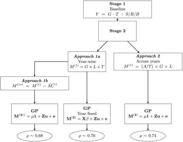
 represents the simple mean of genotypes of the r-th year. In the genomic prediction (GP) stage, M
(2) is the n×1 vector of adjusted means of genotypes by year for Approach 1a and across years for Approach 2, M
(2∗) is the n×1 vector of adjusted means of year effect-corrected genotypes in Approach 1b, X and β are respectively the design matrix and parameter vector of fixed effects, Z is the n×p marker matrix, u is the p-dimensional vector of SNP effects and e the error vector. Y=G·T:S/R/B is the shorthand notation of the model eq. (1) in the text: Y
hijkv=(G
T)hv+S
i+R
ij+B
ijk+e
hijkv, M
(1)=G×L×T stands for the model eq. (2) in the text:
represents the simple mean of genotypes of the r-th year. In the genomic prediction (GP) stage, M
(2) is the n×1 vector of adjusted means of genotypes by year for Approach 1a and across years for Approach 2, M
(2∗) is the n×1 vector of adjusted means of year effect-corrected genotypes in Approach 1b, X and β are respectively the design matrix and parameter vector of fixed effects, Z is the n×p marker matrix, u is the p-dimensional vector of SNP effects and e the error vector. Y=G·T:S/R/B is the shorthand notation of the model eq. (1) in the text: Y
hijkv=(G
T)hv+S
i+R
ij+B
ijk+e
hijkv, M
(1)=G×L×T stands for the model eq. (2) in the text:  , and M
(1)=(A/T)×G×L represents the extended model eq. (4) in the text:
, and M
(1)=(A/T)×G×L represents the extended model eq. (4) in the text:  . The final predictive abilities (ρ) are presented in the ellipses.
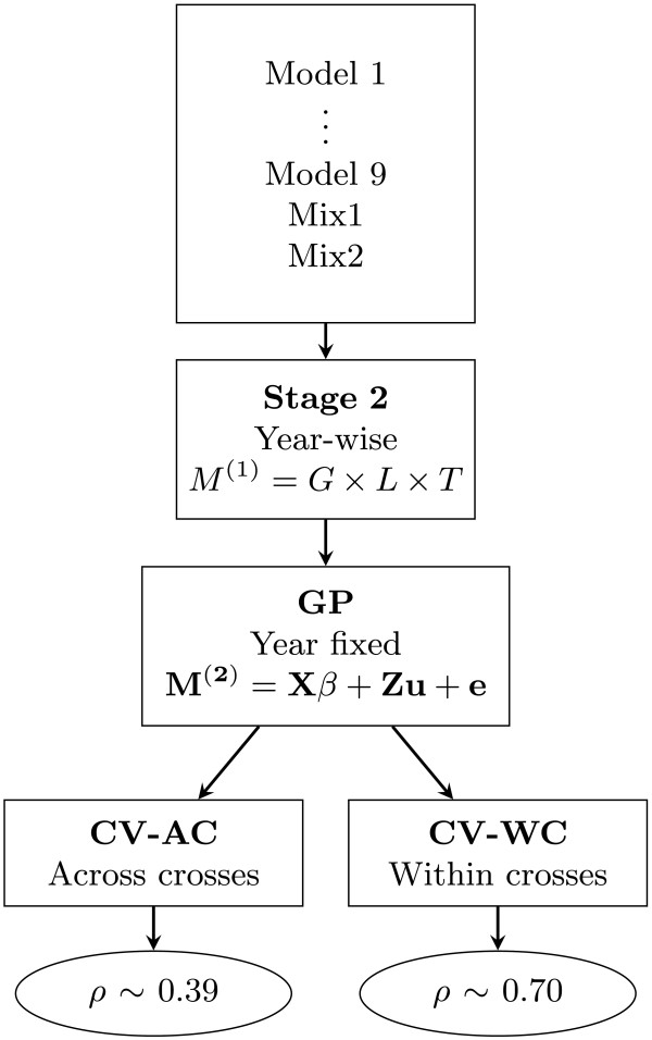
 . In the genomic prediction (GP) stage M
(2) is the adjusted mean of genotypes across locations, X and β are respectively the design matrix and parameter vector of fixed effects, Z is the n×p marker matrix, u is the p-dimensional vector of SNP effects and e the error vector. Sampling methods in cross validation (CV) were across crosses (AC) and within crosses (WC). The final predictive abilities (ρ) are presented in the ellipses.
. In the genomic prediction (GP) stage M
(2) is the adjusted mean of genotypes across locations, X and β are respectively the design matrix and parameter vector of fixed effects, Z is the n×p marker matrix, u is the p-dimensional vector of SNP effects and e the error vector. Sampling methods in cross validation (CV) were across crosses (AC) and within crosses (WC). The final predictive abilities (ρ) are presented in the ellipses.
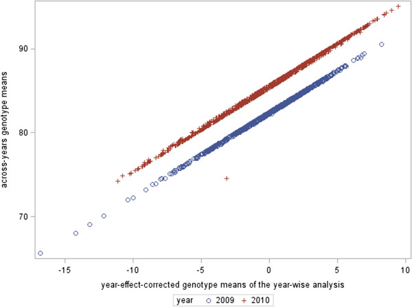
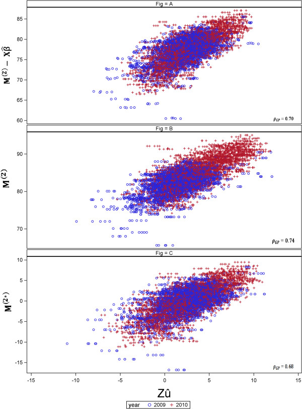
 in (A), M
(2) in (B) and M
(2∗) in (C) ] and the x-axis represents the GEBV (
in (A), M
(2) in (B) and M
(2∗) in (C) ] and the x-axis represents the GEBV ( ). (A) Year-wise analysis (Approach 1a), fitting year as fixed effect in the GP stage, (B) Across-years analysis (Approach 2), using year in the second stage and (C) year-wise analysis using the year effect-corrected genotype means (Approach 1b). ρ
GP represents the predictive ability.
). (A) Year-wise analysis (Approach 1a), fitting year as fixed effect in the GP stage, (B) Across-years analysis (Approach 2), using year in the second stage and (C) year-wise analysis using the year effect-corrected genotype means (Approach 1b). ρ
GP represents the predictive ability.
References
-
- Burgueño J, Crossa J, Cotes JM, San Vicente F, Das B. Prediction assessment of linear mixed models for multienvironment trials. Crop Sci. 2011;51:944–954. doi: 10.2135/cropsci2010.07.0403. - DOI
-
- Piepho HP, Möhring J, Melchinger AE, Büchse A. Blup for phenotypic selection in plant breeding and variety testing. Euphytica. 2008;161:209–228. doi: 10.1007/s10681-007-9449-8. - DOI
Publication types
MeSH terms
LinkOut - more resources
Full Text Sources
Other Literature Sources
Medical
Miscellaneous
