Robust quantification of orientation selectivity and direction selectivity

Abstract

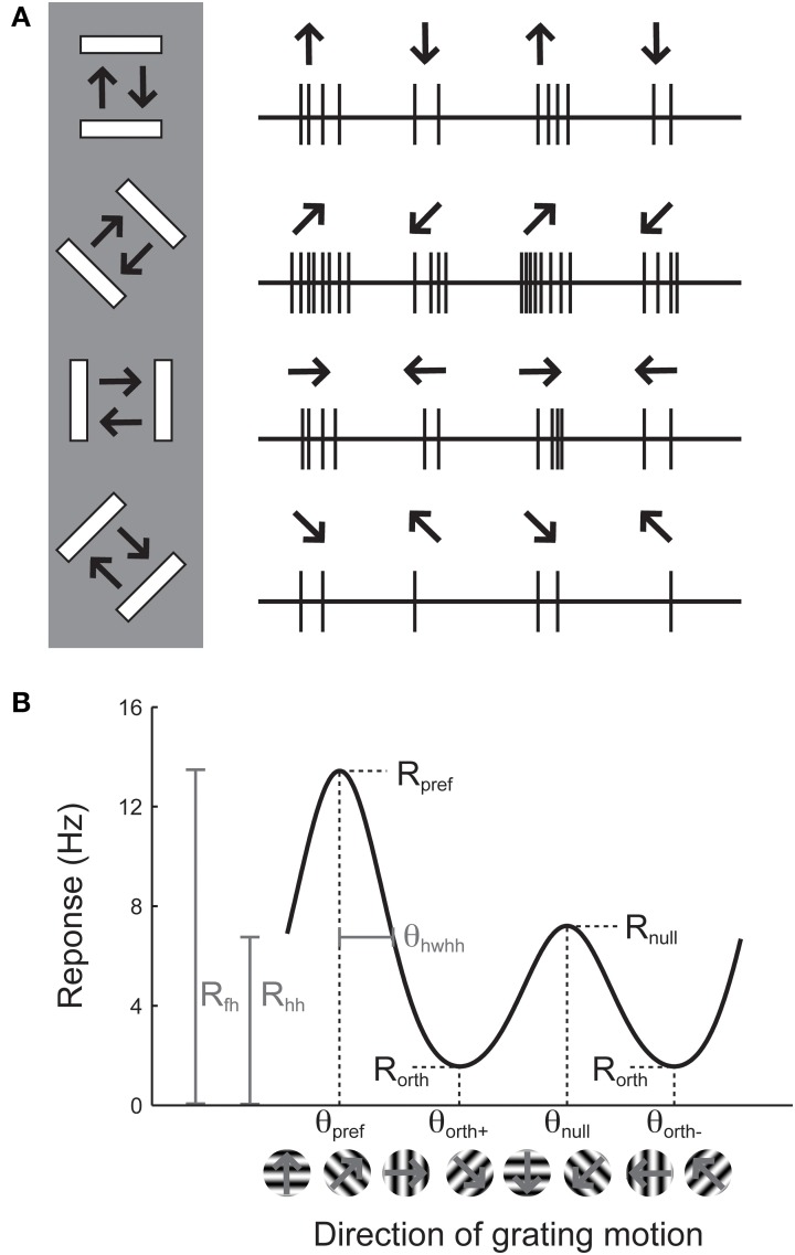
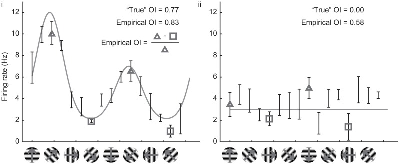
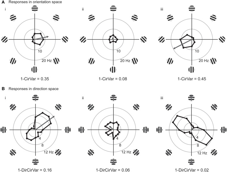
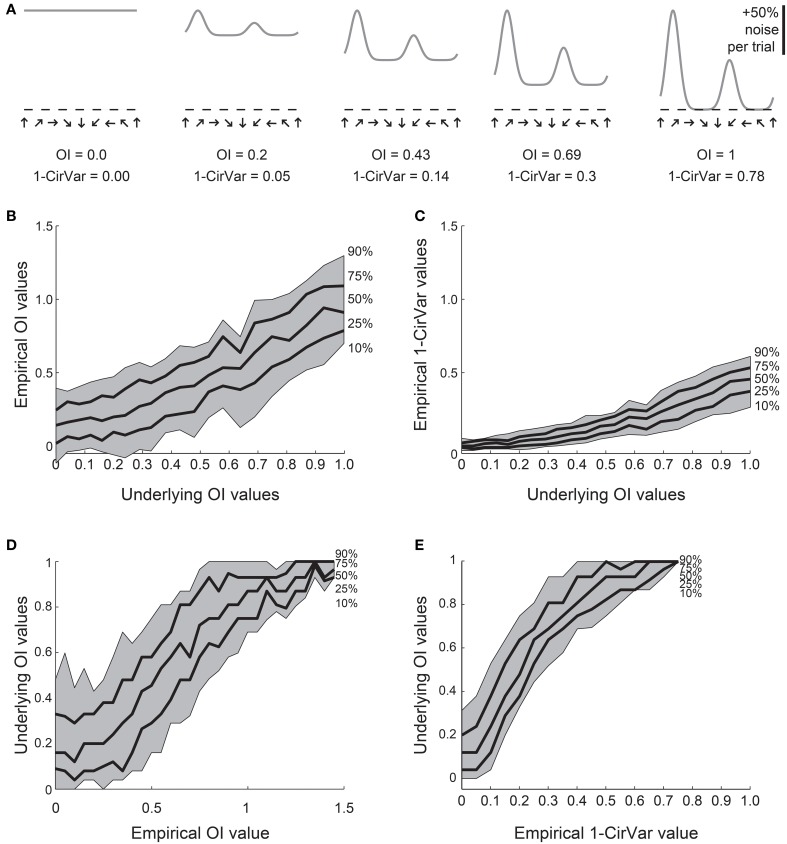
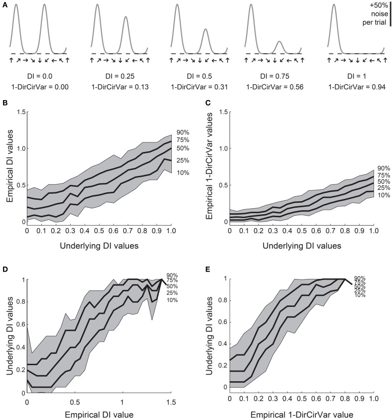
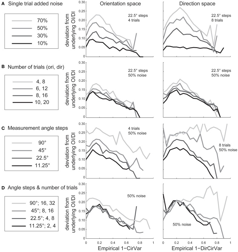
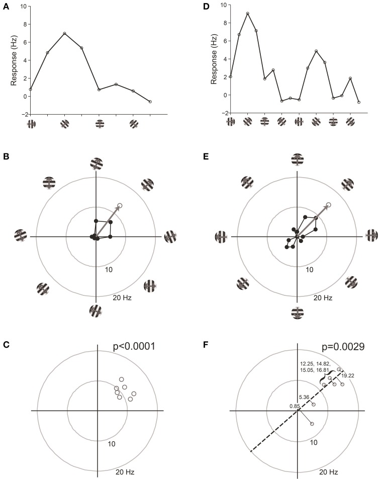
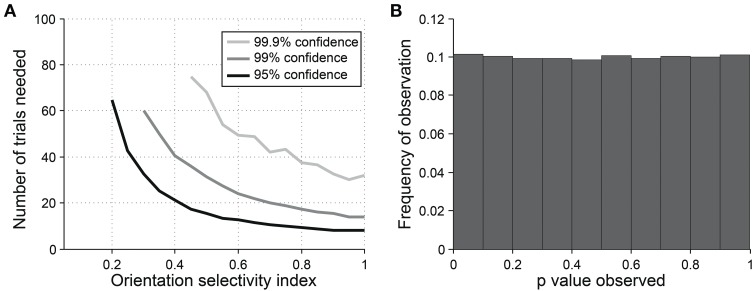
Neurons in the visual cortex of all examined mammals exhibit orientation or direction tuning. New imaging techniques are allowing the circuit mechanisms underlying orientation and direction selectivity to be studied with clarity that was not possible a decade ago. However, these new techniques bring new challenges: robust quantitative measurements are needed to evaluate the findings from these studies, which can involve thousands of cells of varying response strength. Here we show that traditional measures of selectivity such as the orientation index (OI) and direction index (DI) are poorly suited for quantitative evaluation of orientation and direction tuning. We explore several alternative methods for quantifying tuning and for addressing a variety of questions that arise in studies on orientation- and direction-tuned cells and cell populations. We provide recommendations for which methods are best suited to which applications and we offer tips for avoiding potential pitfalls in applying these methods. Our goal is to supply a solid quantitative foundation for studies involving orientation and direction tuning.

Keywords: Monte Carlo; neural data analysis; sampling.

Figure 1

Illustration of the assessment of orientation and direction selectivity. (A) Left: Depiction of a bar stimulus moving at different orientations across the receptive field of an example cell. The cell's responses to each orientation are indicated at the right. The preferred orientation is 45°. During each presentation of the bar stimulus, the stimulus moves back and forth in two opposite directions. This cell responds more strongly to movement of the bar toward 45° than it does to the opposite direction (225°). (B) A graph of responses to the same cell to sinusoidal gratings drifting in several directions. The cell gives the largest response (R_pref) to 45° (θ_pref), and a weaker response (R_null) to the opposite direction 225° (θ_null). The cell responds less strongly to stimulation at either of the two orthogonal orientations (θ_orth+ and θ_orth+). The cell's response decreases as the direction of the stimulus deviates from θ_pref; the difference between θ_pref and the angle that causes the response to drop to half (R_hh) its maximum value is called the half width at half height (θ_hwhh).

Figure 2

Calculation of the empirical orientation selectivity index (OI). (i) Simulated responses (10 trials, 5 Hz per trial noise) to a model cell with an underlying direction tuning curve indicated in gray. Error bars indicate standard error around the mean of the simulated responses. To calculate OI, responses from the preferred orientation angle are averaged together (triangles) and the responses to the orthogonal angles (squares) are subtracted. This quantity is normalized by the response to the preferred orientation angle (triangles). There is good qualitative agreement between the empirical OI and the “true” OI. (ii) Same, for a model cell that is not orientation selective. The empirical OI is still very large due to the noise in the simulated responses, and is not qualitatively similar to the “true” underlying OI.

Figure 3

Responses of model cells in polar coordinates on the complex plane. (A) Responses of model cells in orientation space. Response (in spikes per second) at each angle is indicated by the distance from the origin. Orientation angles vary from 0 (horizontal) to 90° (vertical) and back to 0°/180° (horizontal). Gray arrow indicates the vector mean of the responses to individual orientations. The normalized length of the mean response vector is the quantity L_ori, which is 1 minus the circular variance (1-CirVar). Model cells i and ii are the same as in Figure 2. (B) Responses of the same cells plotted in direction space. Direction of motion is indicated, response at each angle is indicated by the distance from the origin. Note that 0° and 180° both correspond to horizontal stimulus orientations, but moving in upward and downward directions, respectively. Gray arrow indicates the vector mean of responses to individual directions. Note that cell iii is highly orientation selective for oblique bars but is poorly selective for stimulus direction.

Figure 4

Comparison of OI and circular variance measures for simulated data. We created 100 simulations of tuning curves for each of 21 underlying “true” tuning curves, ranging from OI = 0 to OI = 1, some shown in (A). Each trial had 50% noise added. (B) Percentiles of the empirically determined OI for the 100 simulations at each underlying “true” OI value. Note that for cells with 0 true selectivity, the empirical OI values range from slightly negative to almost 0.5. (C) Percentiles of the empirically determined 1-CirVar index for each of the underlying “true” OI values. Note that when “true” OI is low, the 1-CirVar is always low. The index 1-CirVar increases as “true” OI increases but the range of values remains narrower than the corresponding range of empirical OI values in (B). (D) The inverse of (B); given we observed an empirical OI value of x, what is the range of possible “true” OI values that produced x in our simulations? An empirical OI of 0 could have arisen from cells with “true” OI values ranging from 0 to 0.5, and an empirical OI of 0.5 could have arisen from cells with a “true” OI ranging from about 0.1 to about 0.8. (E) The inverse of (C). A 1-CirVar of 0 could have arisen from a “true” OI ranging from 0 to about 0.3, and 1-CirVar of 0.25 could have arisen from a “true” OI ranging from about 0.4 to 0.8. The range of possible underlying “true” OI values is much narrower when 1-CirVar is used as a readout as compared to OI.

Figure 5

Comparison of DI and direction circular variance measures for simulated data. We created 100 simulations of tuning curves for each of 21 underlying “true” tuning curves, ranging from DI = 0 to DI = 1, some curves shown in (A). Each trial had 50% noise added. (B) Percentiles of the empirically determined DI for the 100 simulations at each underlying “true” DI value. Note that for cells with 0 true selectivity, the empirical DI values range from about 0 to about 0.5. (C) Percentiles of the empirically determined 1-DirCirVar index for each of the underlying “true” DI values. Note that when “true” DI is low, the 1-DirCirVar is always low. The index 1-DirCirVar increases as “true” OI increases but the range of values remains narrower than the corresponding range of empirical DI values in (B). (D) The inverse of (B); given we observed an empirical DI value of x, what is the range of possible “true” DI values that produced x in our simulations? An empirical DI of 0 could have arisen from cells with “true” DI values ranging from about 0 to 0.5, and an empirical DI of 0.5 could have arisen from cells with a “true” DI ranging from about 0.1 to 0.7. (E) The inverse of (C). A 1-DirCirVar of 0 could have arisen from a “true” DI ranging from 0 to about 0.4, and 1-DirCirVar of 0.25 could have arisen from a “true” DI ranging from about 0.1 to 0.7. The range of possible underlying “true” DI values is narrower when 1-DirCirVar is used as a readout as compared to DI.

Figure 6

The dependence of error in identifying the true OI on neural noise and stimulus sampling. On the Y axis of all plots is the average deviation between the “true” OI (or DI) and the “best guess” of OI (or DI) based on the empirical 1-CirVar (or 1-DirCirVar). (A) Dependence of error on single trial noise as a percentage of the maximum response rate to the preferred direction. (B) Dependence of error on the number of trials. More trials offer modest improvements in average accuracy. (C) Dependence of error on number of angle steps. Additional angle steps offer a big improvement in estimating the amount of orientation or direction selectivity present. (D) Dependence of error for assorted numbers of trials and angle steps.

Figure 7

Vector-based statistical tests with orientation (A–C) and direction (D–F) responses. This figure uses data from a model cell with strong tuning: Underlying OI = 0.9, DI = 0.5, noise = 20%. 16 directions (22.5° steps) were tested. For the orientation analysis, opposite directions at the same orientation were averaged together. (A) One trial from the model cell plotted in orientation response. Note that a “trial” is defined here as one measurement at each stimulus orientation. (B) The response from the trial shown in (A), plotted in polar coordinates. Black: The response obtained at individual orientations. Gray: The vector sum of the responses at individual orientations. This is the “orientation vector” on this trial. (C) Orientation vectors from seven trials from the model cell. Gray circles show the orientation vectors from the seven trials. The p-value above the graph gives the result of Hotelling's T²-test, which tests for whether the 2-dimensional mean of this distribution of orientation vectors is different from [0, 0]. (D) One trial from the model cell plotted in direction space. Here a “trial” is defined as one measurement at each stimulus direction. (E) The response from the trial shown in (D), plotted in polar coordinates. Gray: The vector sum of the responses at individual directions. This is the “direction vector” on this trial. (F) Direction vectors from seven trials from the model cell. Gray circles show the direction vectors from the seven trials. The dashed line is orientation axis from this cell, obtained by measuring the angle of the average orientation vector. Black lines show the projection of the direction vectors onto the orientation axis (the “direction dot products”). Numbers give the magnitude of the direction dot product for each direction vector. The p-value above the graph gives the result of Student's T-test applied to the direction dot product values against H0: Mean = 0.

Figure 8

Sensitivity and specificity of Hotelling's T-squared test for detecting orientation selectivity. (A) Repeated simulations were performed with a single cell at different levels of underlying OI and different numbers of trials. 16 angles (22.5° steps) were used; noise = 40% at all conditions. Sensitivity of Hotelling's T-squared test was measured at three levels of significance: 95, 99, and 99.9%. For example, the black line shows the number of trials needed such that one would detect an OI difference of X with 95% confidence. (B) A cell was simulated with seven trials at underlying OI = 0. The simulation was repeated 200,000 times and each time a p-value was measured against H0: OI = 0. The frequency of observed p-values was uniform between 0 and 1, which is what would be expected for an unbiased test by repeated sampling of an unoriented cell.

Figure 9

Sensitivity and specificity of the direction dot product test for detecting direction selectivity. (A) Repeated simulations were performed with a single cell at different levels of underlying DI and different numbers of trials; OI = 1 for all simulations. 16 angles (22.5° steps) were used; noise = 4 Hz at all conditions. Sensitivity of the direction dot product test was measured at three levels of significance: 95, 99, and 99.9%. (B) A cell was simulated with 7 trials at underlying DI = 0, OI = 1. The simulation was repeated 200,000 times and each time a p-value was measured against H0: DI = 0. The frequency of observed p-values was uniform between 0 and 1, which is what would be expected for an unbiased test by repeated sampling of cells that are indifferent to direction.

Figure 10

Sensitivity of the 2-sample version of Hotelling's T-squared test for detecting differences preferred orientation between different cell populations. Cells were simulated with seven trials each. We systematically varied the size of the cell populations and the size of the difference in preferred orientation. We measured the sensitivity for detecting the difference at three levels of confidence: 95, 99, and 99.9%. (A) Simulations performed using single-trial noise of 40% in all conditions. (B) Simulations performed using “2-photon OGB-1AM noise”: noise = 20 % + (10% × expected response).

Figure 11

Gaussian fits for assessing orientation and direction selectivity. (A) Common errors with unconstrained fits (gray lines). Left: the unconstrained fit has gotten stuck in a local squared error minimum, using a tiny tuning width to fit 2 points very accurately. Middle: The unconstrained fit has used a peak response R_p that is much larger than any point actually present in the data, and a physiologically implausible negative weight for the null direction. Right: The unconstrained fit has found a reasonable fit, but the parameters do not make physical sense. The unconstrained fit posits a constant offset that is highly negative, with large responses to the preferred and null directions. All of these fitting error can be solved by constraining the fit parameters to values that make physical sense (solid lines, see text). (B) Mean errors in tuning width, preferred angle, and OI for Monte Carlo simulations of cells with the underlying OIs in Figure 4. Gray patch indicates 25–75% interval (C) Mean errors in tuning width, preferred angle, and OI for Monte Carlo simulations of cells with the underlying DIs in Figure 5. Gray patch indicates 25–75% interval.

Figure 12

The dependence of errors in identifying tuning width, preference angle, and OI/DI on neural noise and stimulus sampling. On the Y axis of all plots is the median error between the “true” underlying quantity and the value provided by the fit. (A–C) are in orientation space, and (D–F) are in direction space. (A,D) Dependence of error on single trial noise as a percentage of the maximum response rate to the preferred direction. (B,E) Dependence of error on number of angle steps. Additional angle steps offer a modest improvement in estimating the fit parameters. (C,F) Dependence of error on the number of trials. More trials offer modest improvements in average accuracy.

Figure 13

Estimating the distribution of preferred direction using bootstrap methods. (A) Data from a cell recorded with 2-photon calcium imaging using OGB-1AM before and after extended exposure to a motion stimulus (“motion training”). Bars show ±1 standard error of the response. Solid lines show best fits with double Gaussian functions. The dashed line indicates mean response to a gray screen. (B) Distribution of preferred directions in bootstrap simulations of the cell shown in (A). The data from this cell was randomly resampled with replacement, creating a “simulated” cell, and this simulated data set was fit with double Gaussian functions. This procedure was repeated 100 times in each training condition, yielding the observed distributions of preferred direction. “Unc.” lists the preference uncertainty, meaning the percentage of simulations whose preferred direction differed from the mean direction by more than 90°.

References

1. Batschelet E. (1981). Circular Statistics in Biology. New York, NY: Academic Press
1. Carandini M., Ferster D. (2000). Membrane potential and firing rate in cat primary visual cortex. J. Neurosci. 20, 470–484 - PMC - PubMed
1. Cronin B., Stevenson I. H., Sur M., Kording K. P. (2010). Hierarchical Bayesian modeling and Markov chain Monte Carlo sampling for tuning-curve analysis. J. Neurophysiol. 103, 591–602 10.1152/jn.00379.2009 - DOI - PMC - PubMed
1. De Valois R. L., Yund E. W., Helper N. (1982). The orientation and direction selectivity of cells in macaque visual cortex. Vision Res. 22, 531–544 10.1016/0042-6989(82)90112-2 - DOI - PubMed
1. Garaschuk O., Milos R. I., Grienberger C., Marandi N., Adelsberger H., Konnerth A. (2006). Optical monitoring of brain function in vivo: from neurons to networks. Pflugers Arch. 453, 385–396 10.1007/s00424-006-0150-x - DOI - PubMed