Easy method to examine single nerve fiber excitability and conduction parameters using intact nonanesthetized earthworms

Abstract

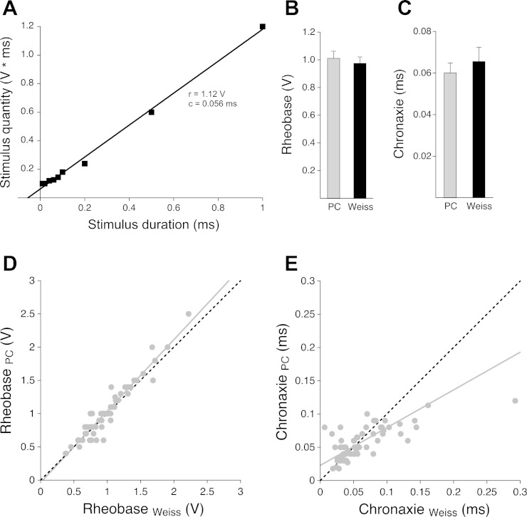
The generation and conduction of neuronal action potentials (APs) were the subjects of a cell physiology exercise for first-year medical students. In this activity, students demonstrated the all-or-none nature of AP generation, measured conduction velocity, and examined the dependence of the threshold stimulus amplitude on stimulus duration. For this purpose, they used the median giant nerve fiber (MGF) in the ventral nerve cord of the common earthworm (Lumbricus terrestris). Here, we introduce a specialized stimulation and recording chamber that the nonanesthetized earthworm enters completely unforced. The worm resides in a narrow round duct with silver electrodes on the bottom such that individual APs of the MGF can be elicited and recorded superficially. Our experimental setup combines several advantages: it allows noninvasive single fiber AP measurements taken from a nonanesthetized animal that is yet restrained. Students performed the experiments with a high success rate. According to the data acquired by the students, the mean conduction velocity of the MGF was 30.2 m/s. From the amplitude-duration relationship for threshold stimulation, rheobase and chronaxie were graphically determined by the students according to Lapicque's method. The mean rheobase was 1.01 V, and the mean chronaxie was 0.06 ms. The acquired data and analysis results are of high quality, as deduced from critical examination based on the law of Weiss. In addition, we provide video material, which was also used in the practical course.

Keywords: Lapicque; Weiss; action potential; chronaxie; conduction velocity; extracellular recording; rheobase.

Fig. 1.

Parameters of electrical threshold stimulation. A: hyperbolic dependence of stimulus amplitude (a) on stimulus duration (t). According to Lapicque, a at a very long stimulus duration is called “rheobase” (r) and t at two times r (2r) is called “chronaxie” (c) (25, 30). The parameters r (and 2r) and c are indicated by dotted lines and arrows. B: linear dependence of stimulus quantity [q; integral of a over t (see inset)] on t according to the law of Weiss (24, 43). The linear graph intersects the y-axis at r × c and the x-axis at (−)c; thus, its slope is r. The formulas in A and B are explained in the appendix. C: the energy (e) of an electrical stimulus has a minimum under chronaxie conditions (14). The graph combines the hyperbolic curve for a with the linear dependence of q to illustrate the derivation of e, which is the product of a and q (14).

Fig. 2.

The common earthworm (Lumbricus terrestris). A schematic drawing of a cross section of Lumbricus is shown. The worm is surrounded by the body wall, which mainly consists of muscle tissue penetrated by two pairs of lateral bristles and two pairs of ventral bristles (setae). Almost all segments contain a pair of nephridia; the gut and three main blood vessels as well as the ventral nerve cord traverse the coelom at almost full length. The median giant nerve fiber and two lateral giant nerve fibers run within the ventral nerve cord.

Fig. 3.

Experimental setup. A: the experimental setup consisted of a stimulator, a data-acquisition unit (connected to a personal computer), and the earthworm chamber. The schematic drawing shows the worm in the chamber with its anterior end on the left where stimulation takes place (stimulus electrodes and ground). Two pairs of recording electrodes in the center of the chamber are connected to the data-acquisition unit, and the alternative places for stimulus or recording electrodes are not in use. B–E: photographs of the earthworm chamber. B: open chamber (lid removed) with a metric plastic ruler to measure distances between electrodes. The rubber strip on the ruler fits between the rubber strips delineating the central “halfpipe” with the electrodes. C: the worm has entered the chamber and is restrained by plugs inserted in the rubber tubings on both sides. D: closed chamber with plugs (syringe needle covers). The chamber is covered with a black lid gently tightened with wing nuts (to avoid escape of the worm and to darken the chamber). E: view from the bottom. The closed chamber has been turned upside down to check whether the worm has contact with all connected stimulation and recording electrodes (see also Supplemental Material for the details of the earthworm chamber).

Fig. 4.

Experimental action potential (AP) generation and signal conduction. A and B: the preset user surface of the data acquisition and analysis software with three horizontal acquisition segments. Channels 1 and 2 show differential recordings from two recording sites, and channel 3 shows the stimulus signal. The time point of stimulation is indicated by the vertical dotted lines (S). A: subthreshold stimulation with a 0.1-ms pulse; stimulus amplitude = 0.9 V. Stimulus artifacts but no AP can be seen in channels 1 and 2. B: suprathreshold stimulation with a 0.1-ms pulse and stimulus amplitude = 1.2 V. The first biphasic AP signals in channels 1 and 2 are caused by the passing through of the median giant nerve fiber AP. C: frequency distribution of stimulus amplitudes determined at stimulus duration = 0.1 ms (bin width: 0.3 V). D: frequency distribution of the conduction velocities (bin width: 3.75 m/s). Conduction velocity was calculated based on the latency difference between the first negative peaks in channels 1 and 2, respectively (time between dotted lines 1 and 2) and the measured distance between the recording electrodes (see Fig. 3B).

Fig. 5.

Rheobase and chronaxie values determined by the students. A: amplitude-duration diagram for threshold stimulation from a typical experiment. The stimulus amplitudes necessary to induce AP firing are plotted against the corresponding stimulus duration on a semilog scale. Due to the logarithmic scaling of the x-axis, the hyperbolic shape of the curve (see Fig. 1A) appears flattened, which facilitates graphic analysis. The dashed line through the data points is a smooth fit that represents the drawing by eye, performed by the students. The dashed leftward pointing arrow represents the asymptote of the curve, which yields the rheobase value (1.2 V in the experiment shown); the dashed downward pointing arrow originates from the point on the curve corresponding to two times rheobase and intersects the x-axis at the chronaxie value (0.054 ms in the experiment shown). B: frequency distribution of rheobase values obtained by the students (bin width: 0.3 V). C: frequency distribution of the corresponding chronaxie values (bin width: 0.015 ms).

Fig. 6.

Critical data examination with the law of Weiss. A: stimulus quantity (integral obtained by multiplying stimulus amplitude by stimulus duration) plotted against stimulus duration (x-axis linear scale). Data are from the same experiment as shown in Fig. 5A. According to the law of Weiss, the integral data were fitted by a linear function of the form q = r × (t + c), derived from q = r × t + r × c (see Fig. 1B), where the slope of the fit is the rheobase (r). Rheobase and chronaxie obtained with the Weiss analysis for the experiment shown are 1.12 V and 0.056 ms, respectively. B and C: comparison of mean rheobase (B) and chronaxie (C) values obtained by students in the practical course (PC) with graphic analysis based on the Lapicque method and from the Weiss analysis (Weiss), respectively; the small difference between the mean rheobase values proved to be significant (P = 0.0161), whereas the mean chronaxie values were not significantly different. D: direct correlation of all individual rheobase values obtained in the practical course (Rheobase_PC) and the corresponding values obtained with the Weiss analysis (Rheobase_Weiss). The continuous gray line represents a linear regression fit to the data points; the dashed black line is a regression assuming 100% correlation (slope of 1 and axis intersept at 0). E: same correlation analysis as in D but for chronaxie values (Chronaxie_PC and Chronaxie_Weiss).

References

1. Bear MF, Connors BW, Paradiso MA. Neuroscience. Baltimore, MD: Lippincott, Williams & Wilkins, 2007.
1. Bostock H, Cikurel K, Burke D. Threshold tracking techniques in the study of human peripheral nerve. Muscle Nerve 21: 137–158, 1998. - PubMed
1. Bostock H, Sears TA, Sherratt RM. The spatial distribution of excitability and membrane current in normal and demyelinated mammalian nerve fibres. J Physiol 341: 41–58, 1983. - PMC - PubMed
1. Brismar T. Electrical properties of isolated demyelinated rat nerve fibres. Acta Physiol Scand 113: 161–166, 1981. - PubMed
1. Bullock TH. Functional organization of the giant fiber system of lumbricus. J Neurophysiol 8: 55–71, 1945.
LinkOut - more resources