Multiscale digital Arabidopsis predicts individual organ and whole-organism growth

Abstract

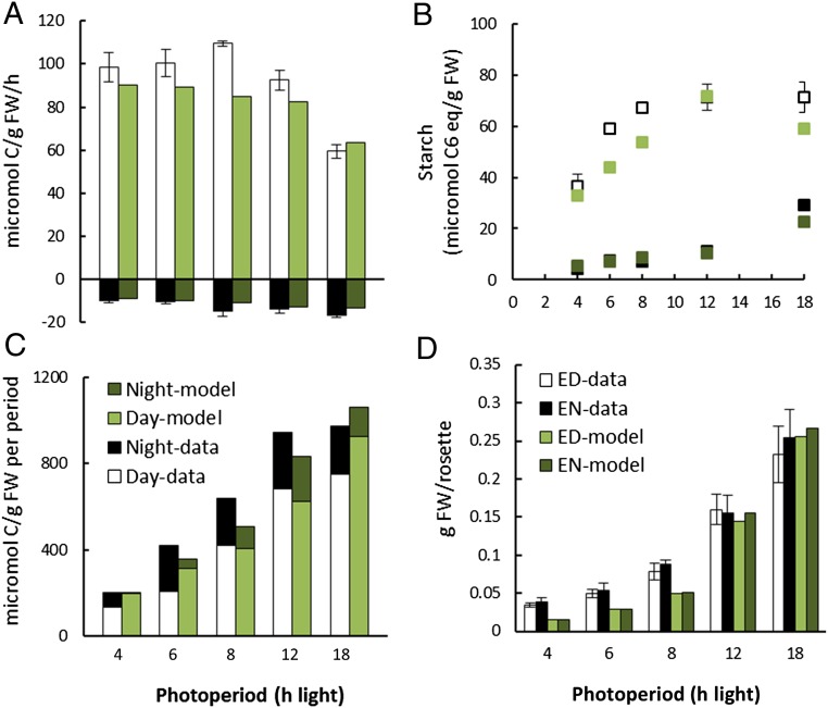
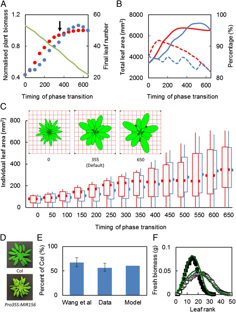
Understanding how dynamic molecular networks affect whole-organism physiology, analogous to mapping genotype to phenotype, remains a key challenge in biology. Quantitative models that represent processes at multiple scales and link understanding from several research domains can help to tackle this problem. Such integrated models are more common in crop science and ecophysiology than in the research communities that elucidate molecular networks. Several laboratories have modeled particular aspects of growth in Arabidopsis thaliana, but it was unclear whether these existing models could productively be combined. We test this approach by constructing a multiscale model of Arabidopsis rosette growth. Four existing models were integrated with minimal parameter modification (leaf water content and one flowering parameter used measured data). The resulting framework model links genetic regulation and biochemical dynamics to events at the organ and whole-plant levels, helping to understand the combined effects of endogenous and environmental regulators on Arabidopsis growth. The framework model was validated and tested with metabolic, physiological, and biomass data from two laboratories, for five photoperiods, three accessions, and a transgenic line, highlighting the plasticity of plant growth strategies. The model was extended to include stochastic development. Model simulations gave insight into the developmental control of leaf production and provided a quantitative explanation for the pleiotropic developmental phenotype caused by overexpression of miR156, which was an open question. Modular, multiscale models, assembling knowledge from systems biology to ecophysiology, will help to understand and to engineer plant behavior from the genome to the field.

Keywords: crop modeling; digital organism; ecology; plant growth model.

Fig. 1.

Overview of the FM. The FM takes environmental data as input (black) to four existing Arabidopsis models (blue shadowed boxes), which are (A) a carbon dynamic model (CDM) that describes carbon assimilation and resource partitioning (31); (B) a functional-structural plant model (FSPM) of individual organ growth that determines the rosette structure (green) and the area for light interception (34); (C) a photothermal model (PTM) that predicts flowering time (1); and (D) a photoperiodism model (PPM), which is a gene dynamic model of the circadian clock and the photoperiod response pathway (6). On integration, several original components were discarded (gray), whereas new connections were created (red).

Fig. 2.

The FM’s workflow predicts whole-plant and individual organ growth data. Input data required are hourly light intensity (A), CO₂ level (B), and temperature (C), illustrated for simulated three 12-h light (open):12-h dark (shaded area) cycles. Carbon supply (D) is used as sugar (dashed line) or stored as starch (solid line). Carbon is allocated at each hourly time step according to the organ demand (E and F). The simulated pattern of demand from individual leaves (F, thin blue lines, left axis) is used to calculate the sum of demand (dots) from leaves (thick blue line, right axis) and roots (brown line, left axis). The root-to-shoot allocation ratio (E), calculated dynamically from the FSPM (red line), is similar to the piecewise-linear function prescribed in the CDM (31) (gray dashed line), which it replaces. Times of dawn and dusk (dots in A) affect the level of flowering gene FT mRNA (G) simulated by the PPM, which in turn controls the accumulation of modified photothermal units (MPTU; H). Once the accumulated photothermal units reach the threshold for flowering (dashed lines), rosette growth is terminated in the FSPM (red arrow). Model outputs include biomass of the shoot (I) and individual leaves (J). Simulations for the Col WT (green lines) closely match experimental data for (I) total shoot biomass, (J) leaf biomass, and (K) leaf area at 18 (○), 25 (●), 27 (□), and 38 (■) d after sowing. Leaves are ranked according to the order of appearance. The integrated model uses simulated sizes of individual leaves (K) to calculate the projected rosette area for photosynthesis (red arrow), considering the spiral leaf arrangement (phyllotaxy) and upward (zenithal) angle. Experimental conditions: ∼21.3 °C; 12:12-h light/dark cycle; light intensity, 110 μmol⋅m⁻²⋅s⁻¹; mean daytime CO₂ level, 375 ppm. The error bars show the SEs of five plants. The color code links to the model components in Fig. 1.

Fig. 3.

The FM predicts plant growth and gas exchange data for different accessions. Model simulations (solid lines) and experimental data (symbols) of total shoot biomass, individual leaf biomass, and leaf number for Ler (A–C) and Fei (D–F) are shown. Time points of measurement in B are 18 (○), 23 (●), 29 (□), and 37 (■) d after sowing (DAS). Time points of measurement in E are 18 (○), 25 (●), and 30 (□) DAS. The thickness of the red lines in C and F represents a region with 1 SD above and below the mean values from the stochastic simulations of leaf number for 2,400 model runs. The plot of modeled and measured NEP of CO₂ is illustrated in G. NEP was measured for plants grown either as a small population on a tray or in individual pots. Experimental conditions: 22 °C; 12:12-h light/dark cycle; light intensity = 130 μmol⋅m⁻²⋅s⁻¹; average daytime CO₂ concentration = 375 ppm. Error bars in A, B, D, and E show the SEs of n = 10 plants for total shoot biomass and n = 5 plants for individual leaf biomass. Error bars in C and F (smaller than the symbols) represent the SD of 24 plants.

Fig. 4.

Testing the FM under different photoperiods. Experimental data (black and white) (51) are compared with model simulations (light and dark green) in the photoperiods indicated, for (A) carbon assimilation and respiration rates; (B) starch levels; (C) amount of growth per day or night period; and (D) rosette fresh weight at the end of day (ED; white and light green) and end of night (EN; black and dark green). Error bars show the SD of five plants.

Fig. 5.

Leaf production rate balances biomass and leaf area for photosynthesis. Simulation results with time-varying leaf production rates (red) and the associated controls with constant rates (blue) are shown for (A) plant biomass (symbols, left axis) and final leaf number at flowering (green line, right axis); biomass is normalized to the maximum value achievable with the varying leaf production rate, which corresponds to a phase transition to the higher, mature rate at 550 degree-days after sowing. (B) Total functional (photosynthesising) leaf area (solid lines, left axis) and percentage of functional leaves (dashed lines, right axis). (C) Boxplots showing the size distribution of functional leaves. Results shown include the minimum and maximum values (whiskers), the first and third quartiles (boxes), and the median values (outer markers). Inset in C illustrates the images of simulated rosettes from the Simile animation tool, for three transition points as indicated under each image. The arrow in A indicates the default (reference) phase transition point in our model. The timing of the phase transition (x axes) are expressed in thermal time after plant emergence. (D) Rosette images of 37-d-old Col WT (Upper) and the greater number of smaller leaves in Pro35S:MIR156 (Lower). (E) Area of the largest leaf in Pro35S:MIR156, relative to Col WT (100%), in the data of Wang et al. (54), our experimental data, and model simulation. Error bars show the SD of five plants in our study. Leaf area in Wang et al. was calculated from published leaf length and width, assuming an elliptical shape. (F) Model simulations (green lines) and experimental data (symbols) of individual leaf biomass in Col (■) and Pro35S:MIR156 (□) at 37 DAS. Experimental conditions: ∼20.7 °C; 12:12-h light/dark cycle; light intensity = 100 μmol⋅m⁻²⋅s⁻¹; average daytime CO₂ concentration = 405 ppm. Error bars show the SEs of five plants.

References

1. Chew YH, et al. An augmented Arabidopsis phenology model reveals seasonal temperature control of flowering time. New Phytol. 2012;194(3):654–665. - PubMed
1. Chapman HW, Gleason LS, Loomis WE. The carbon dioxide content of field air. Plant Physiol. 1954;29(6):500–503. - PMC - PubMed
1. Franklin KA. Light and temperature signal crosstalk in plant development. Curr Opin Plant Biol. 2009;12(1):63–68. - PubMed
1. Michaels SD, Himelblau E, Kim SY, Schomburg FM, Amasino RM. Integration of flowering signals in winter-annual Arabidopsis. Plant Physiol. 2005;137(1):149–156. - PMC - PubMed
1. Corbesier L, et al. FT protein movement contributes to long-distance signaling in floral induction of Arabidopsis. Science. 2007;316(5827):1030–1033. - PubMed
Publication types