. 2014 Sep 10;34(37):12587-600.
doi: 10.1523/JNEUROSCI.1124-14.2014.

Topography and areal organization of mouse visual cortex

Affiliations

Topography and areal organization of mouse visual cortex

Marina E Garrett et al. J Neurosci. .

Abstract

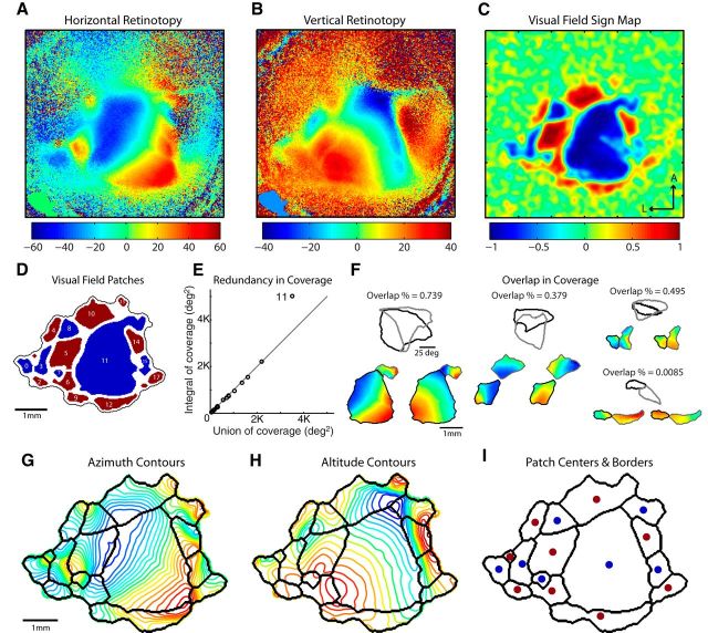
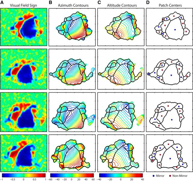
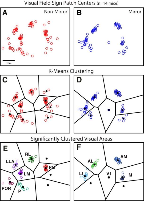
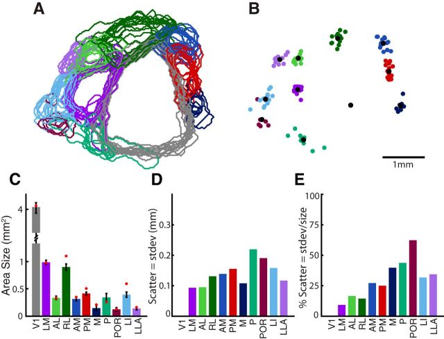
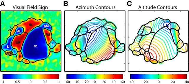
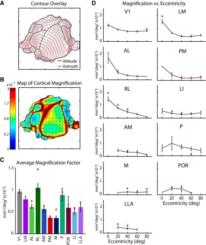
To guide future experiments aimed at understanding the mouse visual system, it is essential that we have a solid handle on the global topography of visual cortical areas. Ideally, the method used to measure cortical topography is objective, robust, and simple enough to guide subsequent targeting of visual areas in each subject. We developed an automated method that uses retinotopic maps of mouse visual cortex obtained with intrinsic signal imaging (Schuett et al., 2002; Kalatsky and Stryker, 2003; Marshel et al., 2011) and applies an algorithm to automatically identify cortical regions that satisfy a set of quantifiable criteria for what constitutes a visual area. This approach facilitated detailed parcellation of mouse visual cortex, delineating nine known areas (primary visual cortex, lateromedial area, anterolateral area, rostrolateral area, anteromedial area, posteromedial area, laterointermediate area, posterior area, and postrhinal area), and revealing two additional areas that have not been previously described as visuotopically mapped in mice (laterolateral anterior area and medial area). Using the topographic maps and defined area boundaries from each animal, we characterized several features of map organization, including variability in area position, area size, visual field coverage, and cortical magnification. We demonstrate that higher areas in mice often have representations that are incomplete or biased toward particular regions of visual space, suggestive of specializations for processing specific types of information about the environment. This work provides a comprehensive description of mouse visuotopic organization and describes essential tools for accurate functional localization of visual areas.

Keywords: extrastriate; imaging; mouse; retinotopy; topography; visual cortex.


Figures

Figure 1.
Figure 1.
Segmentation procedure for delineating visual area patches from retinotopic maps. A, Example map of horizontal retinotopy, in degrees of visual space. The nasal visual field is represented by negative values in blue, transitioning to the temporal periphery with positive values in red. B, Map of vertical retinotopy from the same mouse, in degrees of visual space. The upper field representation is indicated by positive values in red, through the center of space corresponding to the horizontal meridian in green/yellow, and the lower fields at negative values in blue. C, Map of visual field sign computed as the sine of the difference in the angle between the horizontal and vertical map gradients on a pixel-by-pixel basis. Regions having a positive field sign (red) represent nonmirror image transformations of the visual field. A negative field sign (blue) indicates a mirror image representation. Regions with values close to zero lack defined topographic structure. Transitions in field sign between positive and negative values correspond to reversals in the organization of the visual map gradients. Distance between tick marks = 1 mm. D, Thresholded map of visual field sign, revealing discrete patches corresponding to organized topographic maps. E, Scatter plot comparing the integral of coverage to the union of coverage for the identified patches in D. Patches with a redundant representation sit above the unity line, with a ratio of A/AU > 1. Only patch 11 is redundant and was split as shown in F (see left example). F, Assessment of overlap in the visual coverage of each pair of neighboring patches of the same field sign. Retinotopic maps for the two segmented patches are shown in the bottom of the panel. The region of visual space covered by each patch is plotted above, with the value for percentage overlap. Regions showing zero overlap in coverage, such as the bottom right example, were considered to belong to a single area and were fused into a single patch. Overlap greater than zero indicates that the patches were appropriately segmented and that their union would create a redundant representation. G, Patch boundaries overlaid with contour plot of azimuth, corresponding to horizontal retinotopy as in A, with the associated color map. H, Contour plot of altitude lines, corresponding to the map values for vertical retinotopy in B, with patch boundaries overlaid in black. I, Final set of patch boundaries with the CoM of each region labeled according to visual field sign (blue represents mirror; red represents nonmirror).
Figure 2.
Figure 2.
Topography and patch boundaries for individual examples. Each row corresponds to an individual mouse. A, Visual field sign maps computed from vertical and horizontal retinotopy for each case. B, Horizontal retinotopy, shown as azimuth contours, with values indicated by the associated color map. Patch boundaries identified by the segmentation algorithm are overlaid in black. C, Vertical retinotopy, shown as altitude contours, with corresponding color map. Patch boundaries identified by the segmentation algorithm are overlaid in black. D, Borders identified by the segmentation algorithm with the CoM for each patch indicated as blue points for mirror image transformations and red points for nonmirror image representations. Scale is indicated by tick marks, with distance between ticks = 1 mm.
Figure 3.
Figure 3.
Classification of visual areas based on clustering of patch centers after alignment across animals. A, B, Scatter plot of mirror and nonmirror patch centers from each animal, after alignment of the maps across cases using the CoM of the largest patch (i.e., V1) and the direction of its horizontal gradient. Some patch centers fall into visible spatial clusters, whereas others appear more independent. C, D, Voronoi lines (black) illustrate boundaries between k-means clusters. Mean CoM of each cluster is shown as a black dot. E, F, Significant clusters remaining after shuffling analysis (see Materials and Methods). Patches from the more variable clusters were removed from further analysis. Also note that some significant clusters have fewer patches in E and F than in C and D. Patches in significant clusters were removed when there was a closer patch to the cluster's mean CoM, for the same animal. Remaining patch centers are considered reliably identified visual areas, found in a consistent spatial position across animals, labeled and color coded according to their grouping and anatomical position relative to V1. For the set of nonmirror image areas: LM, RL, PM, P, POR, and LLA. For the set of mirror image areas: V1, LI, AL, AM, and M. Tick marks represent 1 mm intervals in scale.
Figure 4.
Figure 4.
Cortical coverage and variability in area position across animals. A, Overlay of all area boundaries across experiments, aligned using V1's CoM and horizontal gradient direction. Areal identity of patch borders was determined according to the classification procedure described in Figure 1. B, Combined scatter plot of visual area centers from all experiments, with each area's mean location in black. C, Average and SE of area size across subjects. D, Scatter in area position for each area. Scatter for each area is defined as the mean distance (mm) between the center locations (colored dots in B) and the average center (black dots in B). Scatter for V1 equals zero because V1's center was used to align all experiments. E, Scatter in area position normalized by area size provides an estimate of how consistently a given area can be found in the same cortical location across animals.
Figure 5.
Figure 5.
Average topographic maps demonstrate features of mouse visual cortical organization. A, Visual field sign map produced by a weighted average of retinotopic maps from all experiments, emphasizing those with stronger responses. The segmentation algorithm was used to identify area boundaries based on retinotopic gradients, as with individual cases. Areal organization of the average map closely corresponds to the layout observed in individual cases, with all major areas identified. B, Average azimuth contours, in degrees, showing progression of the horizontal gradient from temporal fields in red to the nasal field in blue. Area boundaries are shown in black. C, Average altitude contours, in degrees, showing progression of vertical retinotopy from the lower fields in blue to the upper field in red. Area boundaries are in black.
Figure 6.
Figure 6.
Visual coverage of higher areas is often incomplete or biased in space. A, Map of visual eccentricity computed from the average horizontal and vertical retinotopy across animals (Fig. 5). The origin was defined as the intersection of V1, LM, and RL, corresponding to the intersection between the horizontal and vertical meridians. Black lines indicate the computed area borders; white lines indicate iso-contours at 30° and 60°. B, Map of polar angle computed from the average vertical and horizontal retinotopy across animals (Fig. 5). A, B, Tick marks are 1 mm. C, Each panel represents the extent of the visual field covered by each area across cases, with iso-contour lines of eccentricity shown at 0°, 30°, and 90°. Color at each position is the proportion of experiments in which the given visual area showed coverage, limited to the experiments in which the area was found. The coverage profiles from the areas found in the average map (Fig. 5) are also shown as a black contour in each panel. Comparison of visual representations across areas demonstrates differences in the extent and region of visual coverage. D, Average total visual coverage for each identified region. V1 covers a large extent of the visual hemifield, whereas higher areas represent significantly smaller portions of space. E, CoM of visual field coverage profile for each area reveals biases in visual representations toward particular parts of space. F, Each bar represents the proportion of total coverage within each visual field quadrant of the polar coordinate system. Upper quadrants are above the 0° altitude line, and nasal quadrants are in the central 45° of visual space. G, Matrix of visual field overlap between each pair of areas. Coverage overlap was determined as the intersection of coverage, divided by the coverage of the area on the y-axis. Black dots indicate pairs of neighboring areas that have the same visual field sign and were nearby on the cortex.
Figure 7.
Figure 7.
Differences in cortical magnification between areas and across visual eccentricity. A, Overlay of altitude and azimuth contours for the average map illustrating the relationships between vertical and horizontal gradients across cortical space. Contour lines are spaced at 5 degree intervals. B, Cortical magnification computed for each pixel of the average map (in mm2/deg2). An increase in magnification is observed at the lateral V1 border, at the intersection with LM and RL, corresponding to the center of visual space. A, B, Tick marks are 1 mm. C, Magnification averaged across all pixels for each area across cases, with the values for the average map in red. Although the majority of areas have lower magnification compared with V1, as would be expected from having smaller total cortical coverage, a few, notably RL, have similarly high magnification, perhaps associated with their incomplete coverage of visual space, or an emphasis on the nasal visual field. D, Relationship between magnification and visual eccentricity determined for each visual area across cases (black) and in the average map (red). A trend toward higher magnification at central representations is observed for several areas. However, others either lack coverage of the central visual field or show no trend.

References

    1. Andermann ML, Kerlin AM, Roumis DK, Glickfeld LL, Reid RC. Functional specialization of mouse higher visual cortical areas. Neuron. 2011;72:1025–1039. doi: 10.1016/j.neuron.2011.11.013. - DOI - PMC - PubMed
    1. Baizer JS, Ungerleider LG, Desimone R. Organization of visual inputs to the inferior temporal and posterior parietal cortex in macaques. J Neurosci. 1991;11:168–190. - PMC - PubMed
    1. Bleckert A, Schwartz GW, Turner MH, Rieke F, Wong RO. Visual space is represented by nonmatching topographies of distinct mouse retinal ganglion cell types. Curr Biol. 2014;24:310–315. doi: 10.1016/j.cub.2013.12.020. - DOI - PMC - PubMed
    1. Burwell R, Amaral D. Cortical afferents of the perirhinal, postrhinal, and entorhinal cortices of the rat. J Comp Neurol. 1998;205:179–205. - PubMed
    1. Burwell RD. Borders and cytoarchitecture of the perirhinal and postrhinal cortices in the rat. J Comp Neurol. 2001;437:17–41. doi: 10.1002/cne.1267. - DOI - PubMed

Publication types

LinkOut - more resources