An explanatory evo-devo model for the developmental hourglass

Abstract

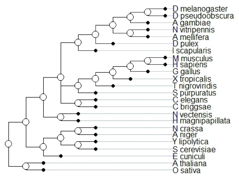
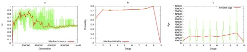
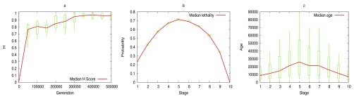
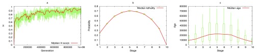
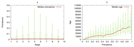
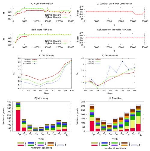
The "developmental hourglass'' describes a pattern of increasing morphological divergence towards earlier and later embryonic development, separated by a period of significant conservation across distant species (the "phylotypic stage''). Recent studies have found evidence in support of the hourglass effect at the genomic level. For instance, the phylotypic stage expresses the oldest and most conserved transcriptomes. However, the regulatory mechanism that causes the hourglass pattern remains an open question. Here, we use an evolutionary model of regulatory gene interactions during development to identify the conditions under which the hourglass effect can emerge in a general setting. The model focuses on the hierarchical gene regulatory network that controls the developmental process, and on the evolution of a population under random perturbations in the structure of that network. The model predicts, under fairly general assumptions, the emergence of an hourglass pattern in the structure of a temporal representation of the underlying gene regulatory network. The evolutionary age of the corresponding genes also follows an hourglass pattern, with the oldest genes concentrated at the hourglass waist. The key behind the hourglass effect is that developmental regulators should have an increasingly specific function as development progresses. Analysis of developmental gene expression profiles from Drosophila melanogaster and Arabidopsis thaliana provide consistent results with our theoretical predictions.

Figure 1.. An abstract DGEN.

( A) The circles denote state-transitioning genes, edges represent directed regulatory interactions, and colored boxes refer to spatial domains that form during development. If regulatory genes become increasingly function-specific as development progresses, the network gradually becomes sparser in that direction. ( B) Evolutionary perturbations on a DGEN’s structure: Gene A is deleted (DL), while gene B is rewired (RW) losing an outgoing edge. This RW event causes the regulatory failure (RF) of gene C, which then causes a cascade of five more RF events. This cascade causes developmental failure (DF). Note that the removal of some upstream regulators does not always cause an RF event (e.g., genes regulated by A).

Figure 2.. Probability of Regulatory Failure (RF) for three values of the parameter z.

r is the fraction of upstream regulating edges that are lost due to a DL or RW event.

Figure 3.. Illustration of the H score calculation.

Let w( l) be the width of stage l. Let w _b be the minimum width across all stages, and suppose that this minimum occurs at stage l = b; this is the waist of the network (ties are broken so that the waist is closer to ⎣ L/2⎦). Consider the sequence X = { w( l)}, l = 1, . . . b} and the sequence Y = { w( l)}, l = b, . . . L}. We denote the normalized univariate Mann-Kendall statistic for monotonic trend on the sequences X and Y as τ _X and τ _Y, respectively. The Mann-Kendall statistic varies between -1 (decreasing) and 1 (increasing), and it is approximately zero for a random sequence. We define H = ( τ _Y − τ _X) /2; H is referred to as the hourglass score. H = 1 if the DGEN is structured as an hourglass, with a decreasing sequence of b stages followed by an increasing sequence of L − b stages. In the computational modeling results, we do not consider the width of the first stage because it can never decrease in Models-1,2,3. We also define a variation of the hourglass score in which we do not take into account adjacent stages in calculating the two Mann-Kendall statistics. That statistic is denoted by $\tilde{H}$ and is referred to as the robust hourglass score.

Figure 4.. The phylotypic tree that we use to calculate the age index of Drosophila’s genes.

Each gene is assigned to one of the following six ages: Level-1: Common ancestor to Fungi, Plants and Eumetazoa. Level-2: Common ancestor to Fungi and Eumetazoa. Level-3: Common ancestor to all Eumetazoa. Level-4: Common ancestor to all Bilateria. Level-5: Common ancestor to all Arthropoda. Level-6: Common ancestor to all Dipteria.

Figure 5.. Computational results with Model-1.

Parameters: 10 runs with different initial populations, N = 10 individuals, L = 10 stages, specificity function s( l) = 0.5 for all stages, Γ = 100 genes at each stage initially, RF parameter z = 4, 1,000,000 generations, probability of RW event P _RW = 10 ⁻⁴. The red line is the median and the green boxes are the 10th, 25th, 75th, and 90th percentiles, across all individuals and all runs. ( a) The hourglass score H across evolutionary time. ( b) Lethality probability at each stage. ( c) Age of existing genes at the last generation.

Figure 6.. Computational results with Model-2.

Parameters: 10 runs with different initial populations, N = 1000 individuals, L = 10 stages, specificity function s( l) = l/L ( l = 1 . . . L − 1), Γ = 100 genes at each stage initially, RF parameter z = 4, 500,000 generations, probability of RW event P _RW = 10 ⁻⁴. The red line is the median and the green boxes are the 10th, 25th, 75th, and 90th percentiles, across all individuals and all runs. ( A) The hourglass score H across evolutionary time. ( B) Lethality probability at each stage. ( C) Age of existing genes at the last generation.

Figure 7.. Computational results with Model-3.

Parameters: 10 runs with different initial populations, N = 10 individuals, L = 10 stages, specificity function s( l) = l/L ( l = 1 . . . L − 1), Γ = 100 genes at each stage initially, RF parameter z = 4, 1,000,000 generations, probability of RW event P _RW = 10 ⁻⁴. The probability of gene duplication P _DP is adjusted dynamically so that the average DGEN size stays between 700 and 800 genes. The red line is the median and the green boxes are the 10th, 25th, 75th, and 90th percentiles, across all individuals and all runs. The hourglass score H across evolutionary time. ( b) Lethality probability at each stage. ( c) Age of existing genes at the last generation.

Figure 8.. Computational results with Model-4.

Parameters: 10 runs with different initial populations, N = 10 individuals, L = 10 stages, specificity function s( l) = l/L ( l = 1 . . . L − 1), Γ = 100 genes at each stage initially, RF parameter z = 4, 1,000,000 generations, probability of RW event P _RW = 10 ⁻⁴. The probability of gene duplication P _DP is adjusted dynamically so that the average DGEN size stays between 700 and 800 genes. The probability of gene deletion (DL) is P _DL = 10 ⁻⁶. The red line is the median and the green boxes are the 10th, 25th, 75th, and 90th percentiles, across all individuals and all runs. ( a) The hourglass score H across evolutionary time. ( b) Lethality probability at each stage. ( c) Age of existing genes at the last generation.

Figure 9.. A nonlinear specificity function, s( l) = 0.9 − 0.8 /(1 + e ^γ−l), for three values of the parameter γ.

This function allows us to control the stage γ at which the specificity is 50%.

Figure 10.. We examine the effect of the two model parameters that affect the location of the DGEN hourglass waist.

The first is the specificity function. To examine its effect, we use a sigmoid-like mathematical function that controls the stage γ at which the specificity is 50% (see Figure 9). This is the stage with the maximum variance in the number of outgoing regulatory edges. RW events at this stage can cause the largest extent of rewiring and so, the highest likelihood of RFs in genes of the next stage. Graph ( a) shows that the location of the hourglass waist is “pushed” towards stage γ, even though it is not always exactly at that stage. The second way to affect the location of the hourglass waist is the parameter z that controls the shape of the RF probability. Increasing z makes RF events more likely, also increasing the likelihood of lethal RF cascades. Graph ( b) shows that as we increase z the hourglass waist moves towards later developmental stages. These results are obtained using Model-2. Parameters: 10 runs with different initial populations, N = 1000 individuals, L = 10 stages, specificity function s( l) = l/L ( l = 1 . . . L − 1), Γ = 100 genes at each stage initially, RF parameter z = 4, 500,000 generations, probability of RW event P _RW = 10 ⁻⁴. The graphs show the median (red lines) and the 10th, 25th, 75th, and 90 ^th percentiles (green boxes) of the location of the waist.

Figure 11.. The prevalence of a gene g in a population of N individuals is the fraction of individuals in which gene g appears.

These results are obtained using Model-2. Parameters: 10 runs with different initial populations, N = 1000 individuals, L = 10 stages, specificity function s( l) = l/L ( l = 1 . . . L −1), Γ = 100 genes at each stage initially, RF parameter z = 4, 500,000 generations, probability of RW event P _RW = 10 ⁻⁴. The graphs show the median (red lines) and the 10th, 25th, 75th, and 90th percentiles (green boxes) for: ( a) prevalence of genes in each stage after 500,000 generations, and ( b) gene age as a function of gene prevalence. As expected, older genes tend to be more prevalent in the population.

Figure 12.. Drosophila results using normalized expression levels.

Graphs ( A) and ( B) show the hourglass score (normal and robust) as a function of the transition threshold c for the two datasets. Graphs ( C) and ( D) show the location of the hourglass waist (stage-pair) as a function of the transition threshold c for the two datasets. Graphs ( E) and ( F) show the Transcriptome Age Index of transitioning genes for three different values of c (chosen so that the number of genes with known age index assigned to each stage is at least 25) for the two datasets. Graph ( G) shows the transitioning genes for the Microarray dataset with c = 0.0005. The transitioning genes constitute 11% of all genes in that dataset. 53% of those genes transition in a single stage-pair. Of the remaining, 64% transition only in consecutive stage-pairs. Note that if a gene transitions n times, it is counted in n stage-pairs. Similarly, graph ( H) shows the transitioning genes for the RNA-Seq dataset with c = 0.00025. The transitioning genes constitute 5% of all genes in that dataset. 45% of those genes transition in a single stage-pair. Of the remaining, 52% transition only in consecutive stage-pairs.

Figure 13.. Arabidopsis thaliana results using normalized expression levels.

Graph ( a) shows the hourglass score (normal and robust) as a function of the transition threshold c. Graph ( b) shows the location of the hourglass waist (stage-pair) as a function of the transition threshold c. Graph ( c) shows the Transcriptome Age Index of transitioning genes for five different values of c (chosen so that the number of genes with known age index assigned to each stage-pair is at least 290). Graph ( d) shows the CDFs of the expression level absolute variations | δ| across successive stage-pairs. Note that in this case the hourglass waist (in terms of number of transitioning genes) appears in stage-pair (3,4), while the oldest genes appear in the next stage-pair. Graph ( e) shows the transitioning genes with c = 0.0001. The transitioning genes constitute 7% of all genes in that dataset. 49% of those genes transition in a single stage-pair. Of the remaining, 36% transition only in consecutive stage-pairs.

Figure S1.. We evaluated the agreement between the two Drosophila datasets in terms of the transitioning genes assigned to each stage-pair, considering only those genes that appear in both datasets.

Because the appropriate transition threshold may be different at each dataset, we use a different threshold for each dataset, say c ₁ and c ₂. For each pair ( c ₁, c ₂), we determine the transitioning genes at each stage-pair with the corresponding dataset., L − 1 pairs of gene sets), and then calculate the average Jaccard similarity across these L − 1 pairs. The Jaccard similarity maps show this average across all stage-pairs for various threshold pairs ( c ₁, c ₂). In graph ( a) with normalized expression levels, when the two thresholds are roughly equal, the average Jaccard similarity is as high as 50%; this means that about 2/3 of the genes assigned to a certain stage-pair using one dataset are also assigned to the same stage-pair using the other dataset. Graph ( b) shows a similar Jaccard similarity map for the case of absolute expression levels. [Dataset 10].

Figure S2.. Drosophila results using absolute expression levels.

Graphs ( a) and ( b) show the hourglass score (normal and robust) as a function of the transition threshold c for the two datasets. Graphs ( c) and ( d) show the location of the hourglass waist (stage-pair) as a function of the transition threshold c for the two datasets. Graphs ( e) and ( f) show the Transcriptome Age Index of transitioning genes for three different values of c (chosen so that the number of genes with known age index assigned to each stage is at least 10) for the two datasets. Graph shows the transitioning genes for the Microarray dataset with c = 5000. The transitioning genes constitute 21% of all genes in that dataset. 62% of those genes transition in a single stage-pair. Of the remaining, 58% transition only in consecutive stage-pairs. Similarly, graph ( h) shows the transitioning genes for the RNA-Seq dataset with c = 10000. The transitioning genes constitute 5% of all genes in that dataset. 45% of those genes transition in a single stage-pair. Of the remaining, 53% transition only in consecutive stage-pairs. [Dataset 11].

Figure S3.. Drosophila data: CDFs of the expression level absolute variations | δ| across successive stage-pairs.

( a) normalized expressions, Microarray, ( b) normalized expressions, RNA-Seq, ( c) absolute expressions, Microarray, absolute expressions, RNA-Seq. [Dataset 12].

Figure S4.. Arabidopsis thaliana results using absolute expression levels.

Graph ( a) shows the hourglass score (normal and robust) as a function of the transition threshold c. Graph ( b) shows the location of the hourglass waist (stage-pair) as a function of the transition threshold c. Graph ( c) shows the Transcriptome Age Index of transitioning genes for five different values of c (chosen so that the number of genes with known age index assigned to each stage-pair is at least 170). Graph ( d) shows the CDFs of the expression level absolute variations | δ| across successive stage-pairs. Graph ( e) shows the transitioning genes with c = 5000. The transitioning genes constitute 8% of all genes in that dataset. 48% of those genes transition in a single stage-pair. Of the remaining, 38% transition only in consecutive stage-pairs. [Dataset 13].

References

1. Raff RA: The shape of life: genes, development, and the evolution of animal form.University of Chicago Press. Trends Ecol Evol. 1996;11(10):441–442. 10.1016/0169-5347(96)81153-0 - DOI
1. Richardson MK, Keuck G: Haeckel’s ABC of evolution and development. Biol Rev Camb Philos Soc. 2002;77(4):495–528. 10.1017/S1464793102005948 - DOI - PubMed
1. Davidson EH: The regulatory genome: gene regulatory networks in development and evolution. Academic Press, 2nd edition.2010. Reference Source
1. Duboule D: Temporal colinearity and the phylotypic progression: a basis for the stability of a vertebrate Bauplan and the evolution of morphologies through heterochrony. Dev Suppl. 1994;1994(Supplement):135–142. - PubMed
1. Rasmussen N: A new model of developmental constraints as applied to the Drosophila system. J Theor Biol. 1987;127(3):271–299. 10.1016/S0022-5193(87)80107-8 - DOI - PubMed
LinkOut - more resources