Lexis diagram and illness-death model: simulating populations in chronic disease epidemiology

Abstract

Chronic diseases impose a tremendous global health problem of the 21st century. Epidemiological and public health models help to gain insight into the distribution and burden of chronic diseases. Moreover, the models may help to plan appropriate interventions against risk factors. To provide accurate results, models often need to take into account three different time-scales: calendar time, age, and duration since the onset of the disease. Incidence and mortality often change with age and calendar time. In many diseases such as, for example, diabetes and dementia, the mortality of the diseased persons additionally depends on the duration of the disease. The aim of this work is to describe an algorithm and a flexible software framework for the simulation of populations moving in an illness-death model that describes the epidemiology of a chronic disease in the face of the different times-scales. We set up a discrete event simulation in continuous time involving competing risks using the freely available statistical software R. Relevant events are birth, the onset (or diagnosis) of the disease and death with or without the disease. The Lexis diagram keeps track of the different time-scales. Input data are birth rates, incidence and mortality rates, which can be given as numerical values on a grid. The algorithm manages the complex interplay between the rates and the different time-scales. As a result, for each subject in the simulated population, the algorithm provides the calendar time of birth, the age of onset of the disease (if the subject contracts the disease) and the age at death. By this means, the impact of interventions may be estimated and compared.

Figure 1. Three states model of normal (healthy), diseased and dead subjects.

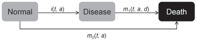
The transition rates may depend on calender time age and in case of also on the duration of the disease.

Figure 2. Three-dimensional Lexis diagram with two life lines.

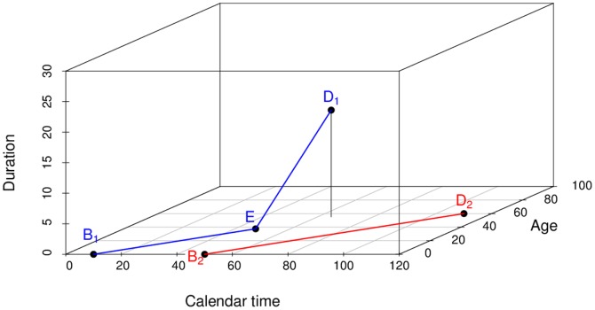
Abscissa, ordinate and applicate (z-axis) represent calendar time , age and duration , respectively. The life lines start at birth and end at death The first subject (blue line segments) contracts the disease at . Then, the life line changes its direction. The second subject (red line segment) does not contract the disease, the life line remains in the t-a-plane.

Figure 3. Theoretical and simulated age-specific prevalence.

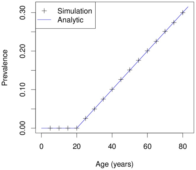
Simulation 1 comprises persons. The resulting age-specific prevalence (black crosses) is compared to the analytically calculated prevalence (blue solid line). The example shows the very good agreement between the simulation and the theoretical results.

Figure 4. Histograms of the age of onset and age at death in a hypothetical chronic disease.

In Simulation 2 the empirical distributions of the age of onset (left) and the age at death of the diseased persons (right) are estimated.

Figure 5. Calculated and simulated prevalence in Simulation 2.

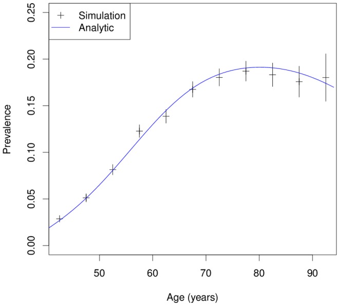
If we mimic a cross-sectional study at year we obtain the age-specific prevalence as indicated by the black bars (with 95% confidence bounds). For comparison the analytically calculated age-specific prevalence is shown as blue line.

Figure 6. Esimtated densities of the gain in life-years in two intervention programmes.

Simulation 4 compares two intervention programmes in a population of 120000 persons. The estimated densities of the total gain in life-years (compared to a basecase) are shown as red and blue curve for programmes A and B, respectively.

References

-
- WHO (2011). Noncommunicable diseases country profiles. URL http://whqlibdoc.who.int/publications/2011/9789241502283eng.pdf. Last access: May 20st, 2014.
- Keiding N (2006) Event history analysis and the cross-section. Statistics in Medicine 25: 2343–2364. - PubMed
- Carstenson B, Kristensen JK, Ottosen P, Borch-Johnsen K (2008) The Danish National Diabetes Register: Trends in Incidence, Prevalence and Mortality. Diabetologia 51: 2187–2196. - PubMed
- Fox C, Sullivan L, Sr RD, Wilson P (2004) The significant effect of diabetes duration on coronary heart disease mortality: the framingham heart study. Diabetes Care 27: 704–708. - PubMed
Publication types
MeSH terms
LinkOut - more resources
Full Text Sources
Other Literature Sources
Medical
Research Materials