A unified design space of synthetic stripe-forming networks

Abstract

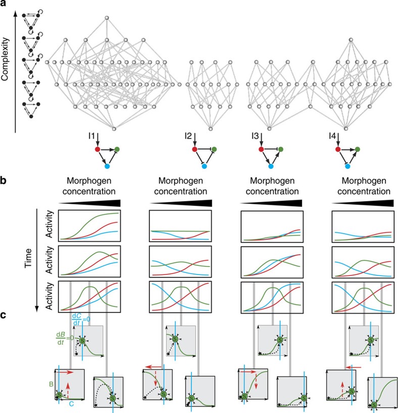
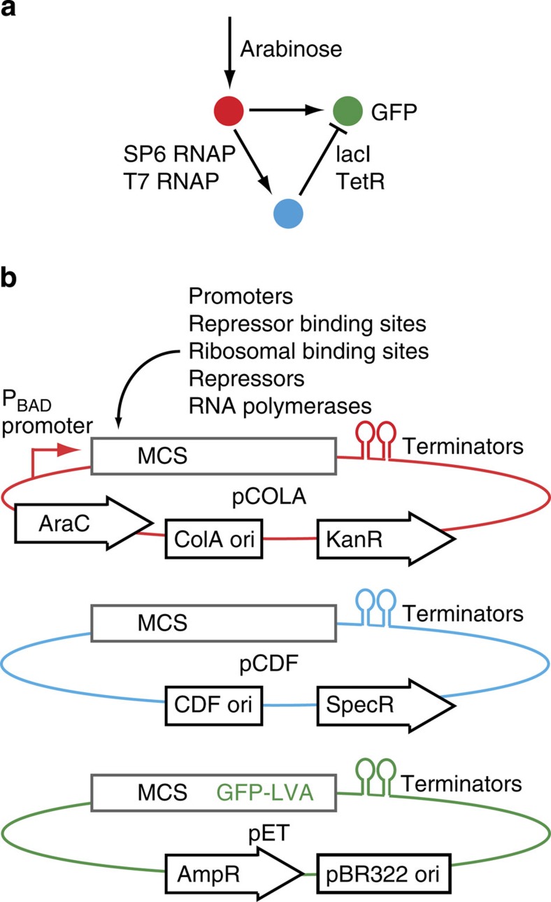
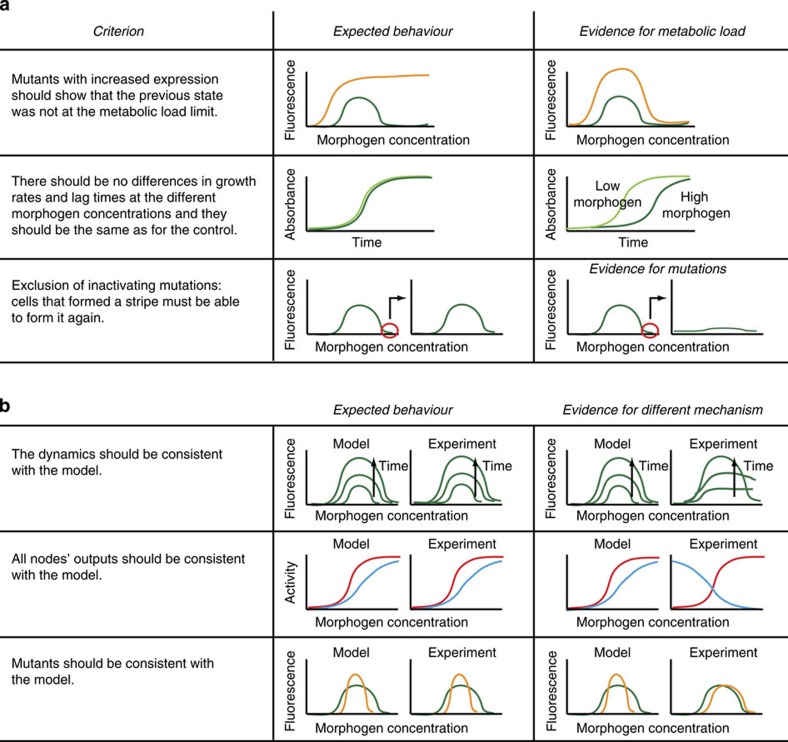
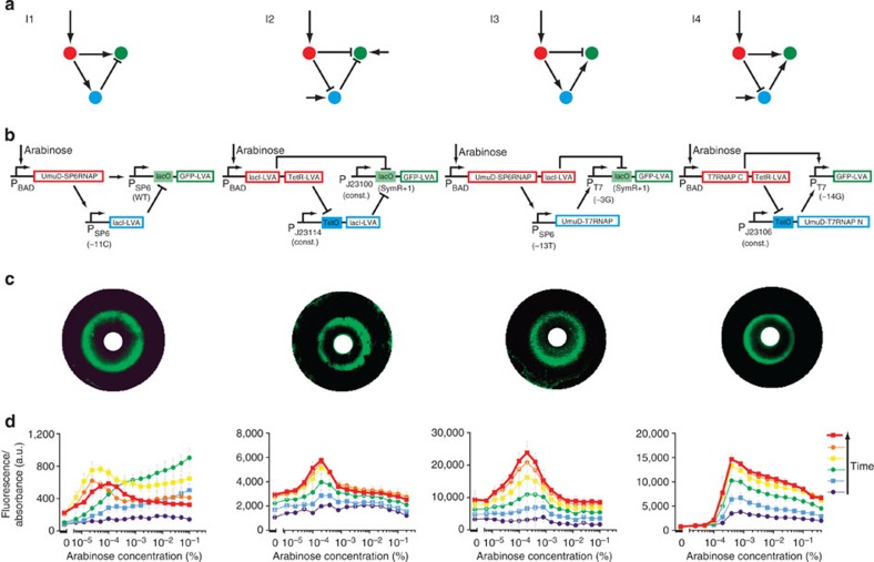
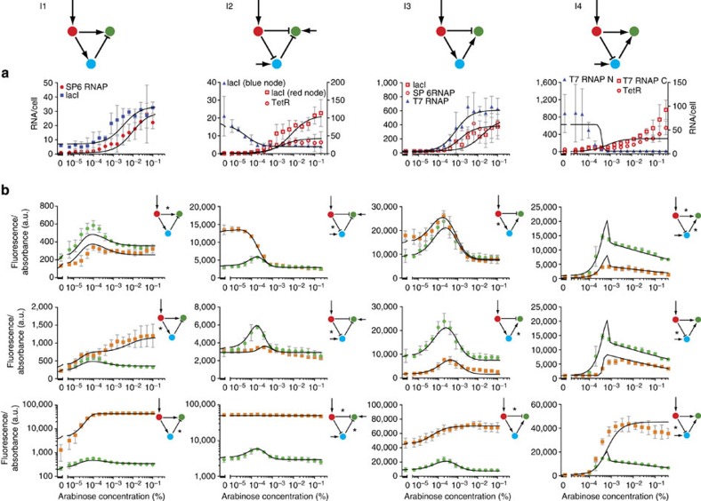
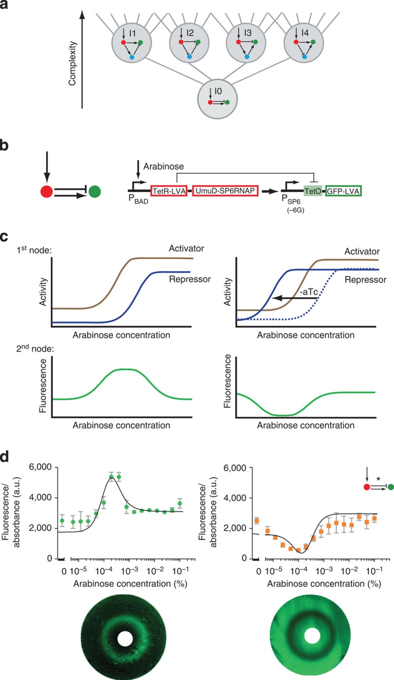
Synthetic biology is a promising tool to study the function and properties of gene regulatory networks. Gene circuits with predefined behaviours have been successfully built and modelled, but largely on a case-by-case basis. Here we go beyond individual networks and explore both computationally and synthetically the design space of possible dynamical mechanisms for 3-node stripe-forming networks. First, we computationally test every possible 3-node network for stripe formation in a morphogen gradient. We discover four different dynamical mechanisms to form a stripe and identify the minimal network of each group. Next, with the help of newly established engineering criteria we build these four networks synthetically and show that they indeed operate with four fundamentally distinct mechanisms. Finally, this close match between theory and experiment allows us to infer and subsequently build a 2-node network that represents the archetype of the explored design space.

Figure 1. Design space of stripe-forming networks.

(a) Complexity atlas: grey circles are gene regulatory networks (GRNs) and edges link those with a single connectivity change. The GRNs are laid out such that complexity increases upwards. Examples of networks with the corresponding number of interactions (complexity) are depicted on the left. The bottoms of the ‘stalactites’ represent minimal networks: the four incoherent feedforward loops (I1-I4). Key: arrow, activation; bar, repression; red, morphogen input receiver gene; blue, intermediate loop gene; green, stripe output gene. (b) The temporal development of the three genes were calculated from representative parameters sets of the complexity atlas and shown schematically for each distinct mechanism. (c) Qualitative phase portraits for each distinct mechanism at low, medium and high morphogen concentration. The x axis represents the activity of the blue gene (that is, C) and the y axis, the activity of the green gene (that is, B). The nullcline curves for the blue and green genes (where one variable does not change in time) are shown as coloured lines, and the stable steady state (S) occurs where they intersect (that is, where neither variable changes over time). The black star indicates the initial condition close to the origin. The full red arrows in these phase plots show the nullcline movements in response to the morphogen gradient and the dashed red arrows indicate the increase or decrease in the height of the nullcline. The calculated temporal trajectories are shown as dashed lines, showing why in some cases a low final level for the green gene is preceded by a temporary rise in levels, while in other cases it is not. It is clear from this analysis that mechanisms cannot be smoothly transformed from one into the other, further highlighting the qualitatively different dynamics for each stalactite.

Figure 2. Network scaffold.

(a) An arabinose-dependent promoter links the concentration-gradient input to a network of activators (T7 and SP6 RNAP) and repressors (lacI and TetR). (b) Each node is encoded on a different E. coli plasmid (color-coded). Each plasmid contains the same multiple cloning sites (MCS) for the combinatorial insertion of the network components. The plasmids contain compatible origins of replication (ori) and antibiotic resistance cassettes (kanamycin, spectinomycin and ampicillin resistance). The 3-node, 3-plasmid scaffold is described fully in Supplementary Methods.

Figure 3. Controls for synthetic stripe-forming circuits in E. coli.

(a) A list of controls or engineering criteria to verify that an observed stripe is not caused by a bacterial stress response to high network expression (metabolic load; Supplementary Fig. 3). (b) A list of controls to verify the mechanism. Green, wild-type network; orange, mutant network; red, morphogen input receiver gene; blue, intermediate loop gene.

Figure 4. The incoherent feedforward loop stripe-forming network family.

(a) The four I-FFLs built (small arrow: constitutive promoter). (b) Implementations of the circuits in the network scaffold (Fig. 2). (c) Bacterial lawns display green fluorescent rings as a function of arabinose gradients from central paper disks (white). (d) E. coli transformed with each network display single fluorescent stripes in arabinose gradients as measured by fluorescence spectrometry (normalized by the absorbance). Time course for I1: 24-min intervals between each sample set, at 4–6 h of growth. For I2, I3 and I4: 12-min intervals, at 5–6 h of growth. Mean and s.d. from three biological replicates.

Figure 5. Quantitative mutant analysis and model fitting.

(a) Measured mRNA concentrations for all genes other than the stripe-forming gene at 6 h of growth. Mean and s.d. from three biological replicates. (b) Comparison of WT (green) and mutant (orange) network fluorescence at 6 h of growth. The interactions marked with an asterisk are modified in the mutant networks. The exact changes and conditions are listed in Supplementary Fig. 7. Mean and s.d. from three biological replicates. The black lines represent the model fitted simultaneously to the RNA data and fluorescence output of the WT and mutant networks for each design class.

Figure 6. Two-node archetypal stripe-forming network (I0).

(a) I0 network complexity shown relative to the I-FFL stripe-forming family. (b) Circuit implementation in the network scaffold. (c) Schematic depictions of archetypal stripe (left) and anti-stripe (right) mechanisms. (d) E. coli transformed with the I0 network display a fluorescent stripe (left) or anti-stripe (right) in arabinose gradients, depending on the aTc concentration (0.125 μM for stripe, 0 μM for antistripe). Mean and s.d. from three biological replicates. The black lines represent the model fitted simultaneously to the RNA data and fluorescence output of the stripe, anti-stripe and a further variant at 5 h of growth (Supplementary Fig. 10). Corresponding bacterial lawns display a fluorescent ring or anti-ring as a function of arabinose gradients from central paper disks (white) (bottom).