Sequence co-evolution gives 3D contacts and structures of protein complexes

Abstract

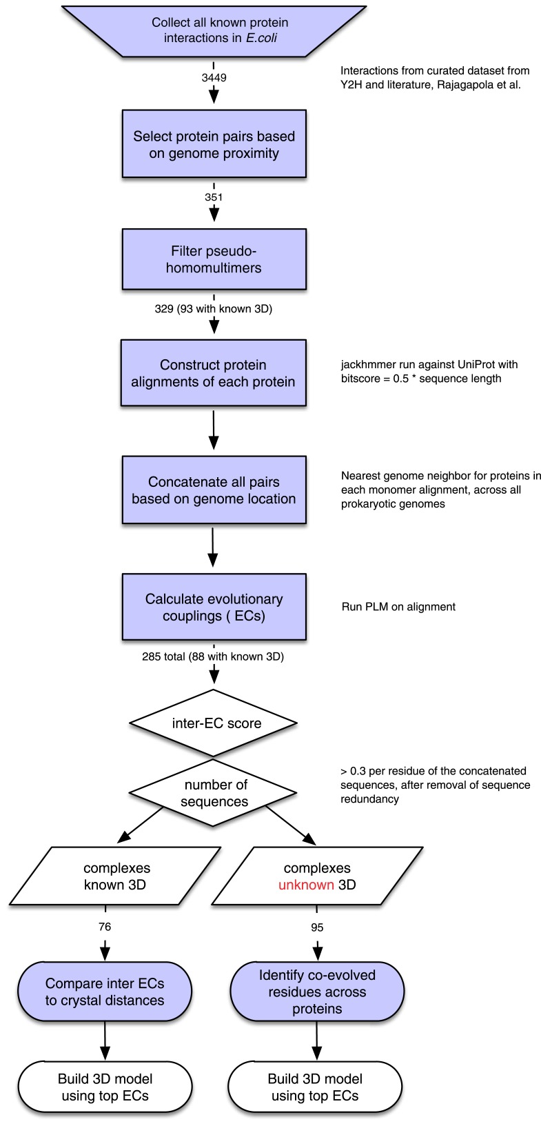
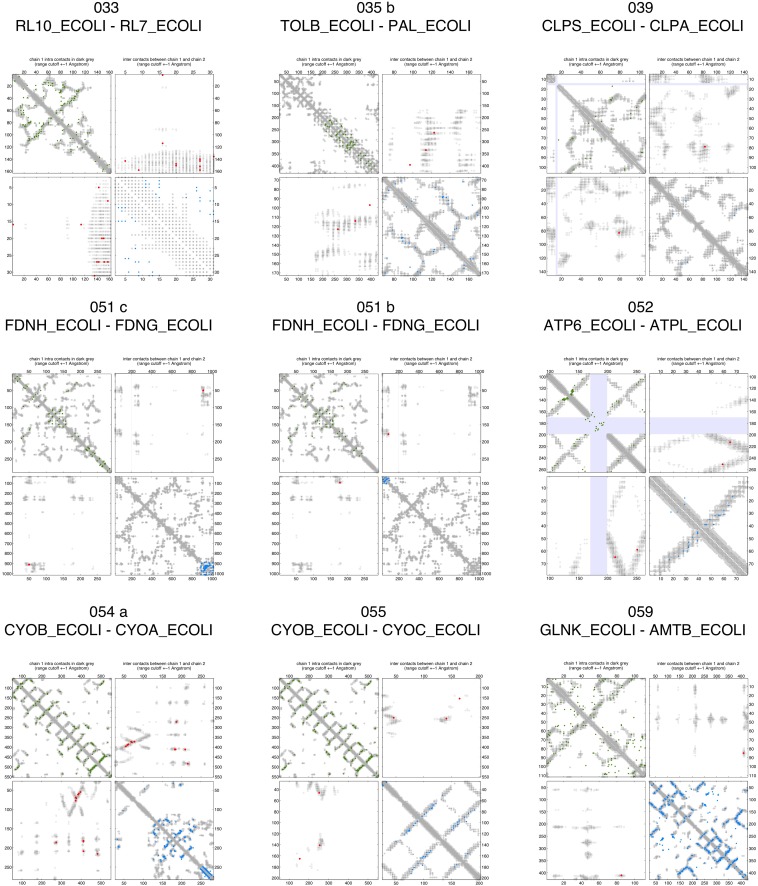
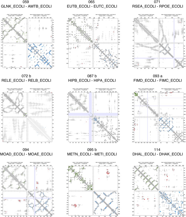
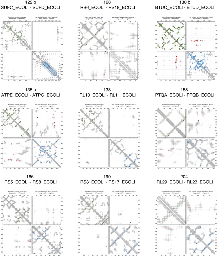
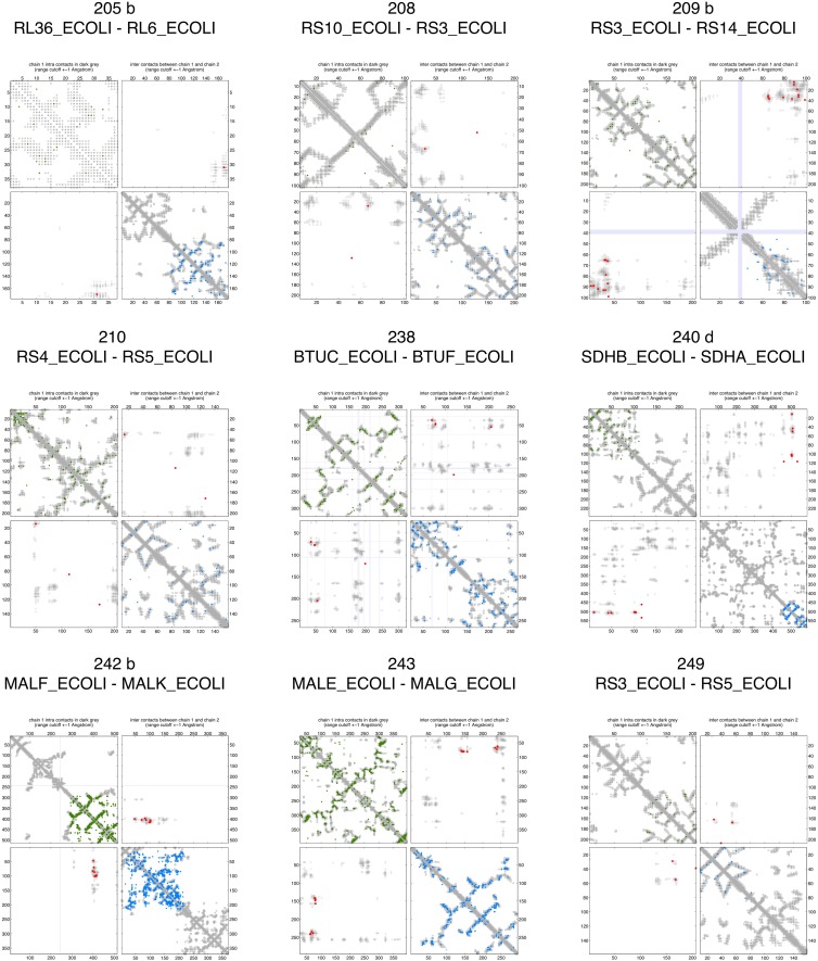
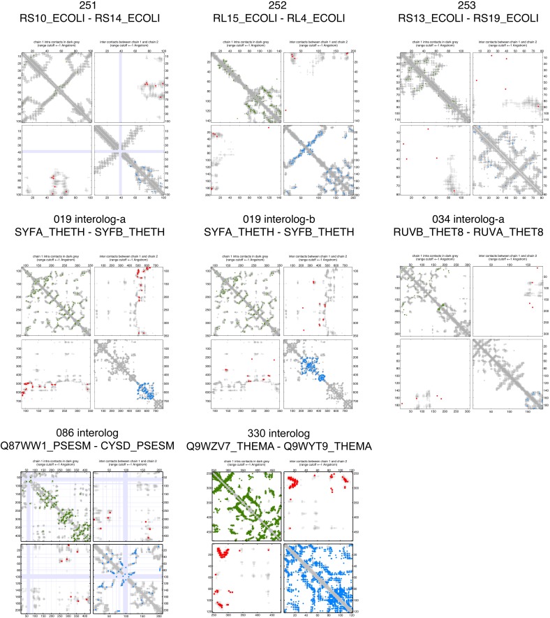
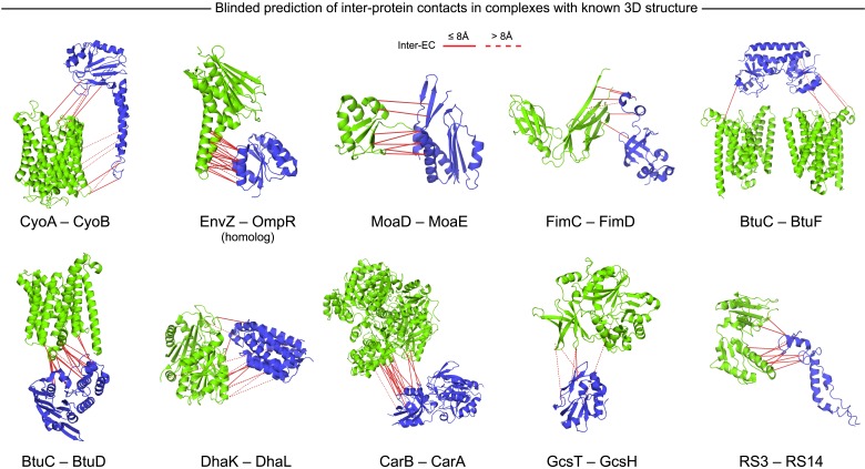
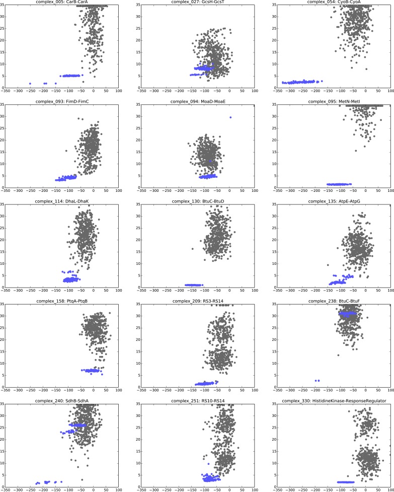
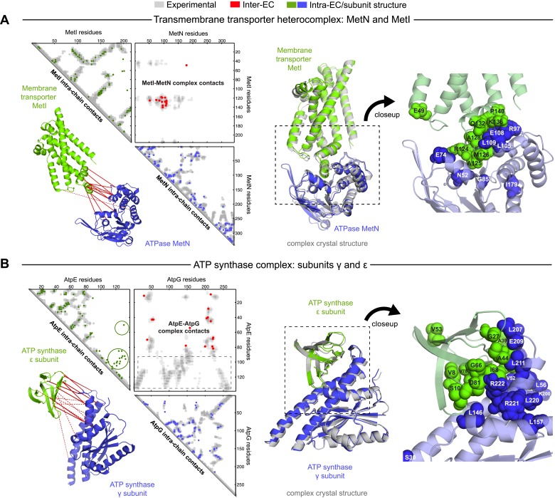
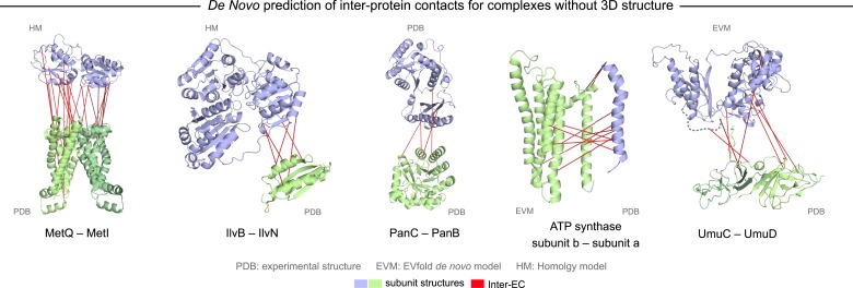
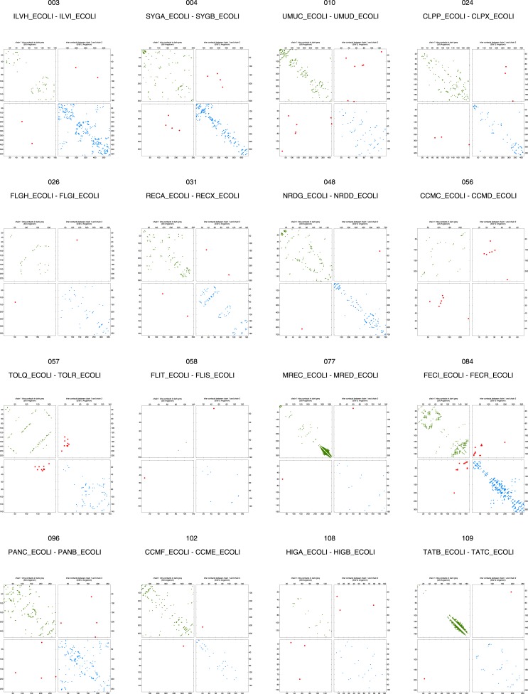
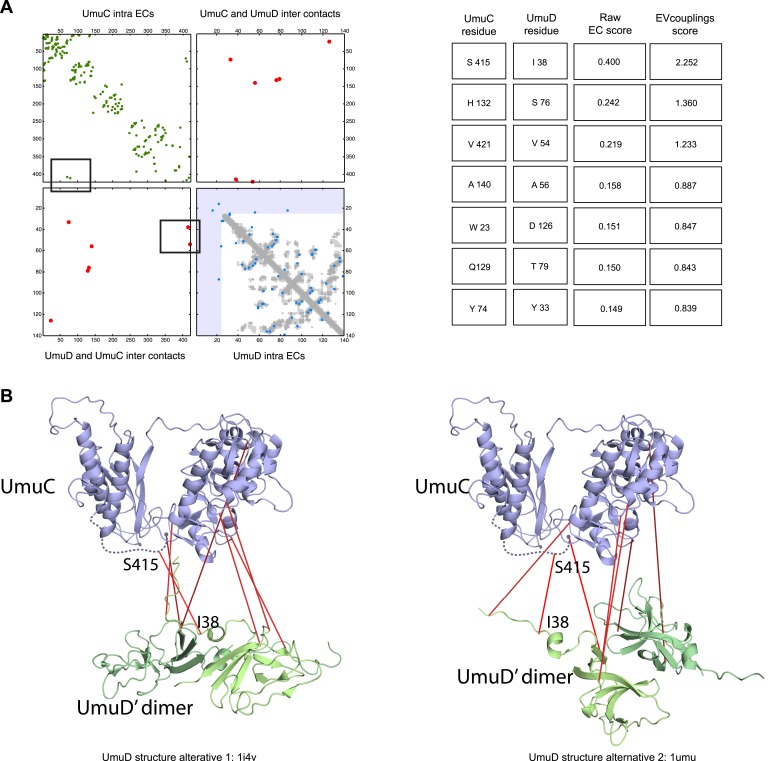
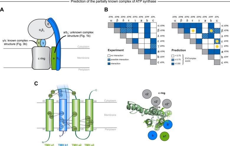
Protein-protein interactions are fundamental to many biological processes. Experimental screens have identified tens of thousands of interactions, and structural biology has provided detailed functional insight for select 3D protein complexes. An alternative rich source of information about protein interactions is the evolutionary sequence record. Building on earlier work, we show that analysis of correlated evolutionary sequence changes across proteins identifies residues that are close in space with sufficient accuracy to determine the three-dimensional structure of the protein complexes. We evaluate prediction performance in blinded tests on 76 complexes of known 3D structure, predict protein-protein contacts in 32 complexes of unknown structure, and demonstrate how evolutionary couplings can be used to distinguish between interacting and non-interacting protein pairs in a large complex. With the current growth of sequences, we expect that the method can be generalized to genome-wide elucidation of protein-protein interaction networks and used for interaction predictions at residue resolution.

Keywords: E. coli; co-evolution; evolutionary biology; genomics; interactions; protein.

Figure 1.. Co-evolution of residues across protein complexes from the evolutionary sequence record.

(A) Evolutionary pressure to maintain protein–protein interactions leads to the co-evolution of residues between interacting proteins in a complex. By analyzing patterns of amino acid co-variation in an alignment of putatively interacting homologous proteins (left), evolutionary couplings between co-evolving inter-protein residue pairs can be identified (middle). By defining distance restraints on these pairs, the 3D structure of the protein complex can be inferred using docking software (right). (B) Distribution of E. coli protein complexes of known and unknown 3D structure where both subunits are close on the bacterial genome (left), allowing sequence pair matching by genomic distance. For a subset of these complexes, sufficient sequence information is available for evolutionary couplings analysis (dark blue bars). As more genomic information is created through on-going sequencing efforts, larger fractions of the E. coli interactome become accessible for EVcomplex (right). A detailed version of the workflow used to calculate all E. coli complexes currently for which there is currently enough sequence information is shown in Figure1—figure supplement 1. DOI: http://dx.doi.org/10.7554/eLife.03430.003

Figure 1—figure supplement 1.. Details of the EVcomplex Pipeline.

DOI: http://dx.doi.org/10.7554/eLife.03430.004

Figure 2.. Evolutionary couplings capture interacting residues in protein complexes.

(A) Inter- and Intra-EC pairs with high coupling scores largely correspond to proximal pairs in 3D, but only if they lie above the background level of the coupling score distribution. To estimate this background noise a symmetric range around 0 is considered with the width being defined by the minimum inter-EC score. For the protein complexes in the evaluation set, this distribution is compared to the distance in the known 3D structure of the complex that is shown here for the methionine transporter complex, MetNI. (Plots for all complexes in the evaluation set are shown in Figure 2—figure supplement 1 and 2.) (B) A larger distance from the background noise (ratio of EC score over background noise line) gives more accurate contacts. Additionally, the higher the number of sequences in the alignment the more reliable the inferred coupling pairs are which then reduces the required distance from noise (different shades of blue). Residue pairs with an 8 Å minimum atom distance between the residues are defined as true positive contacts, and precision = TP/(TP + FP). The plot is limited to range (0,3) which excludes the histidine kinase—response regulator complex (HK–RR)—a single outlier with extremely high number of sequences. (C) To allow the comparison across protein complexes and to estimate the average inter-EC precision for a given score threshold independent of sequence numbers, the raw couplings score is normalized for the number of sequences in the alignment, resulting in the EVcomplex score. In this work, inter-ECs with an EVcomplex score ≥0.8 are used. Note: the shown plot is cut off at a score of 2 in order to zoom in on the phase change region and the high sequence coverage outlier HK-RR is excluded. (D) For complexes in the benchmark set, inter-EC pairs with EVcomplex score ≥0.8 give predictions of interacting residue pairs between the complex subunits to varying accuracy (8 Å TP distance cutoff). All predicted interacting residues for complexes in the benchmark set that had at least one inter-EC above 0.8 are shown as contact maps in Figure 2—figure supplement 3–8. DOI: http://dx.doi.org/10.7554/eLife.03430.005

Figure 2—figure supplement 1.. Distribution and accuracy of raw EC scores for all complexes in evaluation set.

DOI: http://dx.doi.org/10.7554/eLife.03430.006

Figure 2—figure supplement 2.. Distribution and accuracy of raw EC scores for all complexes in evaluation set (2).

DOI: http://dx.doi.org/10.7554/eLife.03430.007

Figure 2—figure supplement 3.. Contact maps of all complexes with solved 3D structure with inter-ECs above EVcomplex score of 0.8.

Predicted coevolving residue pairs with an EVcomplex score ≥0.8 and all inter-ECs up to the rank of the last include inter-EC are visualized in complex contact maps (red dots: inter-ECs, green and blue dots: intra-ECs for monomer 1 and 2, respectively). Top left and bottom right quadrants: intra-ECs; top right and bottom left quadrants: inter-ECs. Inter- and intra-protein crystal structure contacts at minimum atom distance cutoffs of 5/8/12 Å are shown as dark/middle/light gray dots, respectively; missing data in the crystal structure as shaded blue rectangles. DOI: http://dx.doi.org/10.7554/eLife.03430.008

Figure 2—figure supplement 4.. Contact maps of all complexes with solved 3D structure with inter-ECs above EVcomplex score of 0.8 (2).

DOI: http://dx.doi.org/10.7554/eLife.03430.009

Figure 2—figure supplement 5.. Contact maps of all complexes with solved 3D structure with inter-ECs above EVcomplex score of 0.8 (3).

DOI: http://dx.doi.org/10.7554/eLife.03430.010

Figure 2—figure supplement 6.. Contact maps of all complexes with solved 3D structure with inter-ECs above EVcomplex score of 0.8 (4).

DOI: http://dx.doi.org/10.7554/eLife.03430.011

Figure 2—figure supplement 7.. Contact maps of all complexes with solved 3D structure with inter-ECs above EVcomplex score of 0.8 (5).

DOI: http://dx.doi.org/10.7554/eLife.03430.012

Figure 2—figure supplement 8.. Contact maps of all complexes with solved 3D structure with inter-ECs above EVcomplex score of 0.8 (6).

DOI: http://dx.doi.org/10.7554/eLife.03430.013

Figure 3.. Blinded prediction of evolutionary couplings between complex subunits with known 3D structure.

Inter-ECs with EVcomplex score ≥0.8 on a selection of benchmark complexes (monomer subunits in green and blue, inter-ECs in red, pairs closer than 8 Å by solid red lines, dashed otherwise). The predicted inter-ECs for these ten complexes were then used to create full 3D models of the complex using protein–protein docking. For the fifteen complexes for which 3D structures were predicted using docking, energy funnels are shown in Figure 3—figure supplement 1. DOI: http://dx.doi.org/10.7554/eLife.03430.015

Figure 3—figure supplement 1.. Comparison of Interface RMSD to HADDOCK score.

The HADDOCK scores of docked models are plotted against their iRMSDs to the bound complex crystal. Gray data points correspond to models created without any ECs as unambiguous restraints whereas blue dots correspond to model created using all inter-couplings with EVcomplex score ≥0.8. HADDOCK score outliers with scores >100 are not shown, and any model with an iRMSD >35 Å is displayed as iRMSD = 35 Å for visualization purposes. DOI: http://dx.doi.org/10.7554/eLife.03430.016

Figure 4.. Evolutionary couplings give accurate 3D structures of complexes.

EVcomplex predictions and comparison to crystal structure for (A) the methionine-importing transmembrane transporter heterocomplex MetNI from E. coli (PDB: 3tui) and (B) the gamma/epsilon subunit interaction of E. coli ATP synthase (PDB: 1fs0). Left panels: complex contact map comparing predicted inter-ECs with EVcomplex score ≥0.8 (red dots, upper right quadrant) and intra-ECs (up to the last chosen inter-EC rank; green and blue dots, top left and lower right triangles) to close pairs in the complex crystal (dark/mid/light gray points for minimum atom distance cutoffs of 5/8/12 Å for inter-subunit contacts and dark/mid gray for 5/8 Å within the subunits). Inter-ECs with an EVcomplex score ≥0.8 are also displayed on the spatially separated subunits of the complex (red lines on green and blue cartoons, couplings closer than 8 Å in solid red lines, dashed otherwise, lower left). Right panels: superimposition of the top ranked model from 3D docking (green/blue cartoon, left) onto the complex crystal structure (gray cartoon) and close-up of the interface region with highly coupled residues (green/blue spheres). DOI: http://dx.doi.org/10.7554/eLife.03430.017

Figure 5.. Evolutionary couplings in complexes of unknown 3D structure.

Inter-ECs for five de novo prediction candidates without E. coli or interaction homolog complex 3D structure (Subunits: blue/green cartoons; inter-ECs with EVcomplex score ≥0.8: red lines). For complex subunits which homomultimerize (light/dark green cartoon), inter-ECs are placed arbitrarily on either of the monomers to enable the identification of multiple interaction sites. Contact maps for all complexes with unsolved structures are provided in Figure 5—figure supplement 1 and 2. Left to right: (1) the membrane subunit of methionine-importing transporter heterocomplex MetI (PDB: 3tui) together with its periplasmic binding protein MetQ (Swissmodel: P28635); (2) the large and small subunits of acetolactate synthase IlvB (Swissmodel: P08142) and IlvN (PDB: 2lvw); (3) panthotenate synthase PanC (PDB: 1iho) together with ketopantoate hydroxymethyltransferase PanB (PDB: 1m3v); (4) subunits a and b of ATP synthase (model for a subunit a predict with EVfold-membrane, PDB: 1b9u for b subunit), for detailed information see Figure 6; and (5) the complex of UmuC (model created with EVfold) with one possible conformation of UmuD (PDB: 1i4v) involved in DNA repair and SOS mutagenesis. For alternative UmuD conformation, see Figure 5—figure supplement 3. DOI: http://dx.doi.org/10.7554/eLife.03430.018

Figure 5—figure supplement 1.. Contact maps of all complexes without solved 3D structure with at least one inter-ECs above EVcomplex score of 0.8.

Inter-ECs are shown as red dots in the top right and bottom left quadrant while intra-ECs of the two monomers are shown in green and blue in the top left and bottom right quadrant, respectively. DOI: http://dx.doi.org/10.7554/eLife.03430.019

Figure 5—figure supplement 2.. Contact maps of all complexes without solved 3D structure with at least one inter-ECs above EVcomplex score of 0.8 (2).

DOI: http://dx.doi.org/10.7554/eLife.03430.020

Figure 5—figure supplement 3.. Details of the predicted UmuCD interaction residues.

DOI: http://dx.doi.org/10.7554/eLife.03430.021

Figure 6.. Predicted interactions between the a-, b-, and c-subunits of ATP synthase.

(A) The a- and b- subunits of E. coli ATP synthase are known to interact, but the monomer structure of subunits a and b and the structure of their interaction in the complex are unknown. (B) EVcomplex prediction (right matrix) for ATP synthase subunit interactions compared to experimental evidence (left matrix), which is either strong (left, solid blue squares) or indicative (left, crosshatched squares). Interactions that have experimental evidence, but are not predicted at the 0.8 threshold are indicated as yellow dots. (C) Left panel: residue detail of predicted residue–residue interactions (dotted lines) between subunit a and b (residue numbers at the boundaries of transmembrane helices in gray). Right panel: proposed helix–helix interactions between ATP synthase subunits a (green), b (blue, homodimer), and the c ring (gray). The proposed structural arrangement is based on analysis of the full map of inter-subunit ECs with EVcomplex score ≥0.8 (Figure 6—figure supplement 1). DOI: http://dx.doi.org/10.7554/eLife.03430.022

Figure 6—figure supplement 1.. Contact map of predicted ECs in the ATPsynthase a and b subunits.

Inter-ECs are shown as red dots in the top right and bottom left quadrant while intra-ECs of the two monomers are shown in green and blue in the top left and bottom right quadrant, respectively. DOI: http://dx.doi.org/10.7554/eLife.03430.023

Author response image 1.

References

1. Andreani J, Guerois R. Evolution of protein interactions: from interactomes to interfaces. Archives of Biochemistry and Biophysics. 2014;554:65–75. doi: 10.1016/j.abb.2014.05.010. - DOI - PubMed
1. Andreani J, Faure G, Guerois R. InterEvScore: a novel coarse-grained interface scoring function using a multi-body statistical potential coupled to evolution. Bioinformatics. 2013;29:1742–1749. doi: 10.1093/bioinformatics/btt260. - DOI - PubMed
1. Aurell E, Ekeberg M. Inverse Ising inference using all the data. Physical Review Letters. 2012;108:090201. doi: 10.1103/PhysRevLett.108.090201. - DOI - PubMed
1. Baker LA, Watt IN, Runswick MJ, Walker JE, Rubinstein JL. Arrangement of subunits in intact mammalian mitochondrial ATP synthase determined by cryo-EM. Proceedings of the National Academy of Sciences of USA. 2012;109:11675–11680. doi: 10.1073/pnas.1204935109. - DOI - PMC - PubMed
1. Balakrishnan S, Kamisetty H, Carbonell JG, Lee SI, Langmead CJ. Learning generative models for protein fold families. Proteins. 2011;79:1061–1078. doi: 10.1002/prot.22934. - DOI - PubMed
Publication types