Susceptibility-weighted imaging and quantitative susceptibility mapping in the brain

Abstract

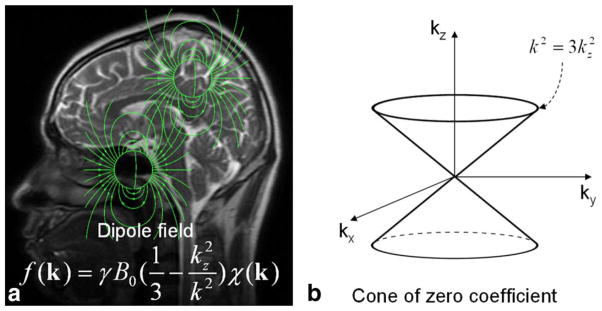
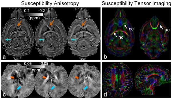
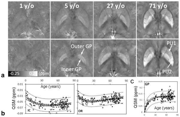
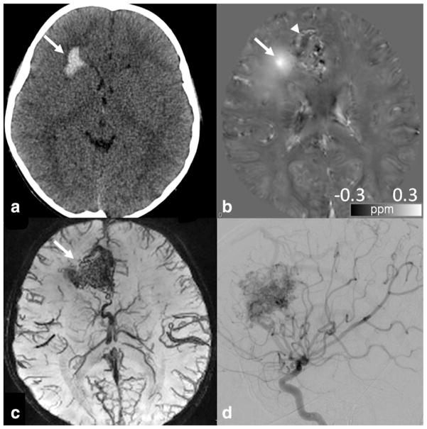
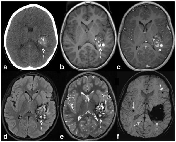
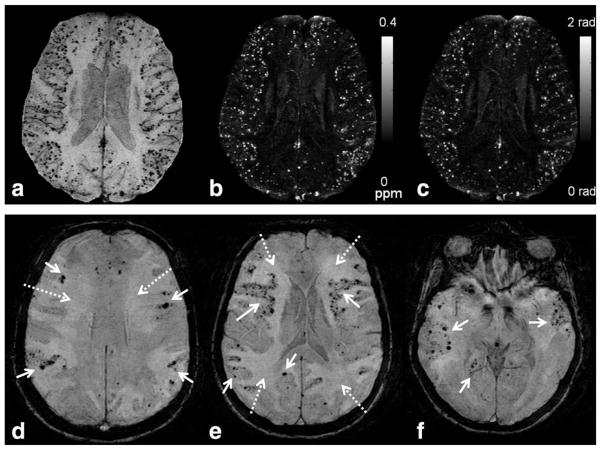
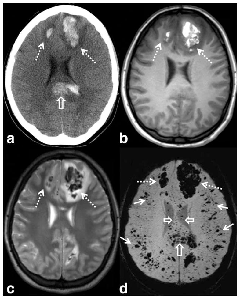
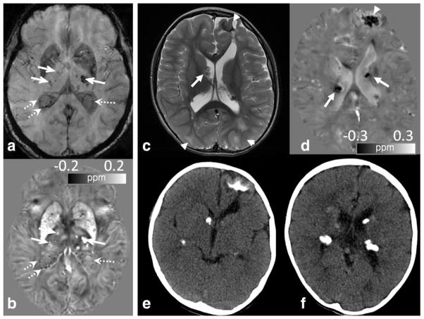
Susceptibility-weighted imaging (SWI) is a magnetic resonance imaging (MRI) technique that enhances image contrast by using the susceptibility differences between tissues. It is created by combining both magnitude and phase in the gradient echo data. SWI is sensitive to both paramagnetic and diamagnetic substances which generate different phase shift in MRI data. SWI images can be displayed as a minimum intensity projection that provides high resolution delineation of the cerebral venous architecture, a feature that is not available in other MRI techniques. As such, SWI has been widely applied to diagnose various venous abnormalities. SWI is especially sensitive to deoxygenated blood and intracranial mineral deposition and, for that reason, has been applied to image various pathologies including intracranial hemorrhage, traumatic brain injury, stroke, neoplasm, and multiple sclerosis. SWI, however, does not provide quantitative measures of magnetic susceptibility. This limitation is currently being addressed with the development of quantitative susceptibility mapping (QSM) and susceptibility tensor imaging (STI). While QSM treats susceptibility as isotropic, STI treats susceptibility as generally anisotropic characterized by a tensor quantity. This article reviews the basic principles of SWI, its clinical and research applications, the mechanisms governing brain susceptibility properties, and its practical implementation, with a focus on brain imaging.

Keywords: MRI, magnetic resonance imaging; MSA, magnetic susceptibility anisotropy; QSM, quantitative susceptibility mapping; STI, susceptibility tensor imaging; SWI, susceptibility weighted imaging; TBI, traumatic brain injury; hemorrhage; iron; multiple sclerosis; myelin; stroke.

Figure 1

A spoiled multiecho gradient echo sequence. Alternating readout polarities are illustrated, although single polarity may also be used. Flow compensation may also be added. The contrast in the magnitude images evolve as the echo time increases due to T₂* decay. Phase values increase as TE increases, thus more phase wraps appear at later echoes. Phase contrast between gray and white matter is still observable under these phase wraps. SWI and QSM may use either single or multiple echoes.

Figure 2

Flowcharts of processing steps of SWI (a) and QSM (b). (a) SWI combines both the magnitude and a filtered phase map in a multiplicative relationship to enhance image contrast. Minimum intensity projection (MIP) is commonly applied to highlight the veins. The contrast can be adjusted by varying the number of slices used in MIP (examples shown in later figures). SWI flowchart adapted from Reichenbach et al (3). (b) There are two major steps involved in QSM: filtering background phase and solving an inverse problem.

Figure 3

Relationship between susceptibility and magnetic field. (a) Each image voxel can be approximated as a magnetic dipole which produces a dipole field that extends beyond the voxel itself. Dipole fields originating from different voxels follow the superposition rule resulting in a convolution relationship between field and susceptibility which can be expressed as a multiplication in the k-space. (b) Solving the inverse problem from field to susceptibility is ill-posed, as the coefficients of the equation become zero on a surface of cone in the k-space when k² = 3k²_z.

Figure 4

Examples of magnetic susceptibility anisotropy and STI in the brain. (a,c) Susceptibility maps measured at three orientations of a mouse brain at 9.4T (a) and a human brain at 3T (c). The values and contrast of the white matter are clearly orientation dependent. Notice that intensity scale is flipped with diamagnetic susceptibility appearing bright. (b,d) Corresponding color-coded eigenvector maps calculated by STI. Imaging parameters at 9.4T are: 3D SPGR, matrix size = 256 × 256 × 256, FOV = 22 × 22 × 22 mm³, flip angle = 60°, TE = 8 msec, and TR = 100 msec, 19 orientations. Parameters at 3T are: flow-compensated 3D SPGR, TE = 40 msec, TR = 60 msec, flip angle = 20°, FOV = 256 × 256 × 256 mm², matrix size = 128 × 128 × 128, 16 orientations.

Figure 5

QSM of brain development and aging. (a) Susceptibility values and contrast evolve as a function of age. Brain nuclei become more paramagnetic (hyperintense) as the age increases. Gray and white matter contrast also increases overall. (b) Susceptibility is diamagnetic in the white matter. It first decreases, becoming more diamagnetic during brain development and maturation, followed by an increase as the brain ages. (c) In the nuclei, susceptibility increases monotonically following an exponential function of age. IC, internal capsule; OR, optical radiation; GP, globus pallidus. The scan parameters are: in-plane resolution = 0.9 × 0.9 mm², matrix = 256 × 208, flip angle = 20°, TE of first echo = 4.92 msec, echo spacing = 4.92 msec, TR = 35 msec, and number of echoes = 6. The slice thickness is 2 mm.

Figure 6

An 8-year-old boy with hemorrhage from an ateriovenous malformation. (a) CT obtained at presentation showed right frontal lobe hemorrhage (arrow). (b) QSM obtained at 3T shortly after the CT showed bright signal abnormality, confirming the presence of iron/hemorrhage (arrow). Additional areas of curvilinear and nodular bright signal was seen medial to the lesion, possibly suggesting additional areas of hemorrhage, thromboses, or abnormal vasculature or draining vein containing deoxyhemoglobin (arrowhead). GRE sequence parameters are: 3D multiecho EPI, flip angle 20°, 1 × 1 × 1 mm³, BW 62.50 kHz, TR = 59.3 msec, TE = 13, 28, 43 msec. (c) SWI minIP image demonstrated abnormal vascular tangle typical of arteriovenous malformation (arrow). (d) Final diagnosis of arteriovenous malformation was confirmed by cerebral angiogram.

Figure 7

A 5-year-old boy presented with a large cerebellar developmental venous anomaly (DVA). (a) Multiple linear, branching low signal abnormality is seen in the left cerebellum on SWI minIP image, suggestive of DVA (arrow). Low signal abnormality in the brainstem associated with enhancement (not shown) representing telangiectasia (arrowhead) is also noted. (b) Cerebral angiogram confirmed characteristic feature of DVA in this patient, including a large draining venous stalk (arrow). (c) QSM also identifies dominant draining venous stalk (arrowhead) and multiple anomalies veins (arrows) as bright signal, likely due to presence of deoxyhemoglobin. SWI/QSM protocol is the same as Fig. 6.

Figure 8

SWI is very sensitive to slow flow vascular malformations such as cerebral cavernous malformations (CCM), as in this child with a large left temporal CCM (dashed arrows), with a characteristic “popcorn” appearance on CT and MRI. There are typical internal calcifications on CT (a), hyperintense subacute blood products on T₁WI (b), mild internal enhancement on postcontrast T₁WI (c), and peripheral hypointense hemosiderin on FLAIR (d) and T₂WI (e). The lesion appears larger on SWI (f) due to blooming artifact. More important, additional smaller CCMS are detected (solid arrows), which indicate that the patient likely has multiple familial CCM syndrome (which can occur in as many as 1/3 of patients with CCM). SWI parameters are: 3T, TE = 20 msec, TR = 29 msec, FA = 15°, FOV 250 mm × 188 mm, matrix 448 × 336, 2 mm thick acquisition displayed with 16 mm minIP.

Figure 9

SWI can play an important role in diagnosing cerebral amyloid angiopathy (CAA) and changing patient management. Microbleeds in CAA are in contrast to those from chronic hypertension, which are typically located in the deeper structures such as the deep white matter, deep gray nuclei, or brainstem. These microbleeds were not visible on any other imaging sequence or modality. These patients are at risk for intracranial hemorrhage and should avoid anticoagulation therapy. (a) Numerous tiny microbleeds are seen on SWI, scattered throughout the cortex of the cerebral hemispheres (white arrows) in this elderly patient, typical for CAA. These lesions are also well visualized on maximum intensity projection of QSM (b) and filtered phase maps (c). Projection was made through 8 slices each of 2-mm thickness. Note that the small veins are shown most clearly on the SWI image, less clearly on the phase, and even less so on the QSM projection. Imaging parameters are: 1.5T, TE = 35ms, TR = 85ms, 512 × 512 × 64 acquisition matrix, BW = 160 Hz/pixel, ETL = 5, FA = 25° and acquisition time roughly 8 minutes. (a–c) Courtesy of Saifeng Liu and E. Mark Haacke. (d–f) A 73-year-old patient presented with progressive encephalopathy. SWI shows numerous microbleeds in a cortical pattern (solid arrows), likely due to cerebral amyloid angiopathy (CAA). Patchy edema was also present (dashed arrows), suggestive of CAA-related inflammation. (d–f) Image parameters were: 1.5 T, TE = 40 msec, TR = 57 msec, FA = 20°, FOV 256 × 256, matrix 512 × 512, 2 mm thick acquisition, and 16 mm thick minimal intensity projection.

Figure 10

SWI can provide important information in the setting of stroke, as in this 50-year-old male who presented with acute dissection and occlusion of the right internal carotid artery in the neck. Diffusion-weighted image (a) showed a small infarct in the right frontal white matter (dashed white arrow) Parametric map of mean transit time, from dynamic-contrast enhanced MR perfusion (b) showed a large area of delayed perfusion (large white arrows) in the right MCA territory, demarcating a large penumbra. SWI image at the level of the circle of Willis (c) showed abnormal hypointense signal in the right MCA (open white arrow) compared to the normal hyperintense signal in the left MCA (open black arrow), indicating slow flow or intravascular thrombus or markedly elevated intra-arterial deoxyhemoglobin. SWI image at the level of the lateral ventricles (d) showed markedly prominent cortical and deep medullary veins in the right hemisphere (small solid white arrows), matching the penumbra. The prominent veins indicate high levels of deoxyhemoglobin, indicating increased oxygen extraction. SWI parameters are: 3T, TE = 20 msec, TR = 29 msec, FA = 15°, FOV 230 mm × 172 mm, matrix 448 × 336, 2 mm thick acquisition displayed with 16 mm minIP.

Figure 11

SWI has shown higher sensitivity to traumatic microhemorrhages, particularly in the setting of diffuse axonal injury. Images from a young patient involved in a motor vehicle accident shows large hemorrhagic contusions in the frontal lobes (dashed arrows) on CT (a), T₁-WI (b), T₂-WI (c), and SWI (d). A large hemorrhagic shearing injury in the corpus callosum is also visible on CT, but more extensive involvement is visible on SWI (open arrows). Widespread traumatic microhemorrhages throughout the gray–white matter junction are only visible on SWI (solid white arrows). SWI parameters are: 3T, TE = 20 msec, TR = 29 msec, FA = 15°, FOV 250 mm × 188 mm, matrix 448 × 336, 2 mm thick acquisition displayed with 16 mm minIP.

Figure 12

QSM can differentiate calcification from iron deposit and veins. (a,b) An elderly volunteer shows numerous hypointense spots in the thalamus (solid arrows) and in the ventricles (dotted arrows) adjacent to veins and choroid plexus on T₂*-weighted images (a). QSM (b) reveals hypointense calcifications (dotted arrows) in the ventricles which are clearly differentiated from the adjacent veins and iron deposition in the thalamus. (c–f) An 8-month-old male infant with tuberous sclerosis and multiple calcified dysplasias and hamartomas. (c) Numerous cortical/subcortical tubers, or dysplasias, (arrowhead) and subependymal nodules (arrows) were seen on the T₂ FSE image. (d) Corresponding QSM image revealed dark signal associated with many of these lesions, which would be expected for calcification but not iron (arrows and arrowhead). SWI/QSM protocol of (c,d) is the same as Fig. 6. (e,f) This was confirmed by CT.

Figure 13

A 49-year-old multiple sclerosis patient. (a) MS plaques are usually best visualized on FLAIR images. (b) Hyperintense lesions on FLAIR may exhibit increased magnetic susceptibility on the QSM images (arrows). The sizes and boundaries of hyperintense lesions appear differently on QSM. This increased susceptibility may indicate demyelination and or iron deposition. (c) SWI without minIP shows the perivenular distribution of the lesions and venous involvement. SWI and QSM may provide greater understanding of the pathophysiology of the disease. SWI/QSM parameters are: in-plane resolution = 0.9 × 0.9 mm², matrix = 256 × 208, flip angle = 20°, TE of first echo = 4.92 msec, echo spacing = 4.92 msec, TR = 35 msec, and number of echoes = 6. The slice thickness is 2 mm. [Color figure can be viewed in the online issue, which is available at wileyonlinelibrary.com.]

References

1. Haacke EM, Xu Y, Cheng YC, Reichenbach JR. Susceptibility weighted imaging (SWI) Magn Reson Med. 2004;52:612–618. - PubMed
1. de Crespigny AJ, Roberts TP, Kucharcyzk J, Moseley ME. Improved sensitivity to magnetic susceptibility contrast. Magn Reson Med. 1993;30:135–137. - PubMed
1. Reichenbach JR, Venkatesan R, Schillinger DJ, Kido DK, Haacke EM. Small vessels in the human brain: MR venography with deoxyhemoglobin as an intrinsic contrast agent. Radiology. 1997;204:272–277. - PubMed
1. de Rochefort L, Brown R, Prince MR, Wang Y. Quantitative MR susceptibility mapping using piece-wise constant regularized inversion of the magnetic field. Magn Reson Med. 2008;60:1003–1009. - PubMed
1. Shmueli K, de Zwart JA, van Gelderen P, Li TQ, Dodd SJ, Duyn JH. Magnetic susceptibility mapping of brain tissue in vivo using MRI phase data. Magn Reson Med. 2009;62:1510–1522. - PMC - PubMed
Publication types