CanvasDB: a local database infrastructure for analysis of targeted- and whole genome re-sequencing projects

Abstract

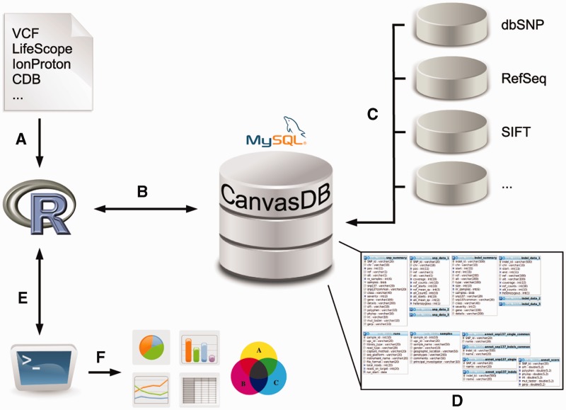
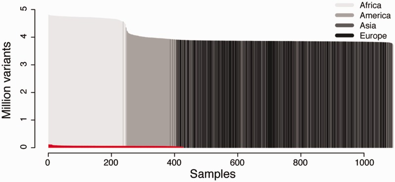
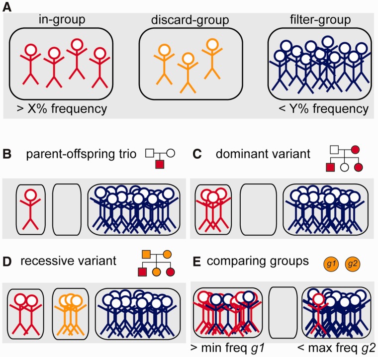
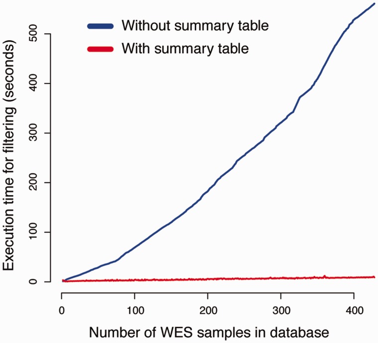
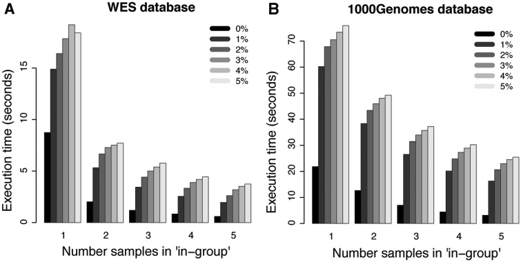
CanvasDB is an infrastructure for management and analysis of genetic variants from massively parallel sequencing (MPS) projects. The system stores SNP and indel calls in a local database, designed to handle very large datasets, to allow for rapid analysis using simple commands in R. Functional annotations are included in the system, making it suitable for direct identification of disease-causing mutations in human exome- (WES) or whole-genome sequencing (WGS) projects. The system has a built-in filtering function implemented to simultaneously take into account variant calls from all individual samples. This enables advanced comparative analysis of variant distribution between groups of samples, including detection of candidate causative mutations within family structures and genome-wide association by sequencing. In most cases, these analyses are executed within just a matter of seconds, even when there are several hundreds of samples and millions of variants in the database. We demonstrate the scalability of canvasDB by importing the individual variant calls from all 1092 individuals present in the 1000 Genomes Project into the system, over 4.4 billion SNPs and indels in total. Our results show that canvasDB makes it possible to perform advanced analyses of large-scale WGS projects on a local server. Database URL: https://github.com/UppsalaGenomeCenter/CanvasDB.

Figure 1.

Overview of the canvasDB system. The figure shows a schematic view of the workflow how variant data are imported, stored and analyzed within the canvasDB system. (A, B) Variant calls for SNP are added to the system using a function call in R; different file formats are supported. (C) All new variants that are not already stored within the system are annotated against databases like dbSNP, RefSeq, SIFT, etc. (D) The variant data, annotations and information about the samples are stored in MySQL database tables, in a way that allows for rapid comparative analyses of variants between samples. (E) Analysis on the variants within the canvasDB system is performed through functions in R, using the RMySQL package. (F) Using pre-defined or custom analysis functions in R/Bioconductor, it is possible to generate lists of candidate disease-causing mutations, or any other types of analysis results, statistics or graphical plots based on the variant data in the database.

Figure 2.

Datasets used for testing the performance of canvasDB. The figure shows the number of individuals (x-axis) and number of variants (y-axis) in the 1000 Genomes data and 428 locally produced WES samples. The 1000 Genomes samples are colored in different shades of gray for populations on different continents. The WES samples are colored in red. All samples have been ordered for each of the datasets with the individuals having the highest number of variants furthest to the left.

Figure 3.

Schematic representation of the variant filtering function. (A) All individuals in the database are divided into three distinct groups; the ‘in-group’ (to the left, in red), ‘discard-group’ (in the middle, orange) and ‘filter-group’ (to the right, blue). The function then returns all SNPs or indels in the system that are detected in at least X% of the ‘in-group’ and at the same time at most Y% of the ‘filter-group’. Individuals in the ‘discard-group’ are excluded from the analysis. With this filtering function, it is possible to perform many different types of filtering, as shown in the examples below. (B) Filtering to detect a de novo mutation in a child of a sequenced mother–father–child trio. (C) Detection of a dominant variant in a family. (D) Detection of a recessive variant in a family. In this case, family members that may be healthy carriers are put in the ‘discard-group’. (E) Detection of variants that occur with frequency of at least X% in one group of samples (‘in-group’, g1) and at least Y% in all other samples (‘filter-group’, g2).

Figure 4.

Summary tables speed up the variant filtering. The graphs show the execution times for a simple filtering query (y-axis) as a function of the number of WES samples in the database (x-axis). The task was to detect all variants that were shared by two individuals in the WES database, while absent from all other individuals. The blue line shows the performance of a naïve method that does not use the summary tables for filtering. When summary tables are used the execution time can be dramatically reduced, at least for larger database sizes, as indicated by the red line.

Figure 5.

Filtering performance for WES and WGS datasets. Each bar in the plots shows the average execution time for 10 filterings with randomly selected individuals in the ‘in-group’. The five different groups of bars in each of the panels show the results when 1, 2, 3, 4 and 5 individuals are present in the ‘in-group’, respectively. The different shades of gray corresponds to results where at most 0%, 1%, 2%, 3%, 4% and 5% of the individuals in the ‘filter-group’ were allowed to carry the variant. (A) Results for filterings in the WES database. (B) Results for filterings in the 1000 Genomes WGS database.

Figure 6.

Visualization of 10 000 Genomes data in a specific region. The colored lines show the Minor Allele Frequencies (MAF) in different 1000 Genomes populations for 28 SNPs on a haplotype, denoted haplotype D, over the FADS region on chromosome 11. At the top are the transcript isoforms of FADS1 and FADS2. Red vertical lines mark the genomic positions of the 28 SNPs on haplotype D. Haplotype frequency varies between populations having ancestry on different continents, with lowest MAF seen in populations with African ancestry and highest MAF in American populations.

References

1. de Ligt J., Willemsen M.H., van Bon B.W., et al. (2012) Diagnostic exome sequencing in persons with severe intellectual disability. N. Engl. J. Med., 367, 1921–1929 - PubMed
1. Rauch A., Wieczorek D., Graf E., et al. (2012) Range of genetic mutations associated with severe non-syndromic sporadic intellectual disability: an exome sequencing study. Lancet, 380, 1674–1682 - PubMed
1. Abecasis G.R., Altshuler D., Auton A., et al. (2010) A map of human genome variation from population-scale sequencing. Nature, 467, 1061–1073 - PMC - PubMed
1. Li Y., Vinckenbosch N., Tian G., et al. (2010) Resequencing of 200 human exomes identifies an excess of low-frequency non-synonymous coding variants. Nat. Genet., 42, 969–972 - PubMed
1. Schuster S.C., Miller W., Ratan A., et al. (2010) Complete Khoisan and Bantu genomes from southern Africa. Nature, 463, 943–947 - PMC - PubMed
Publication types