Properties of selected mutations and genotypic landscapes under Fisher's geometric model

Abstract

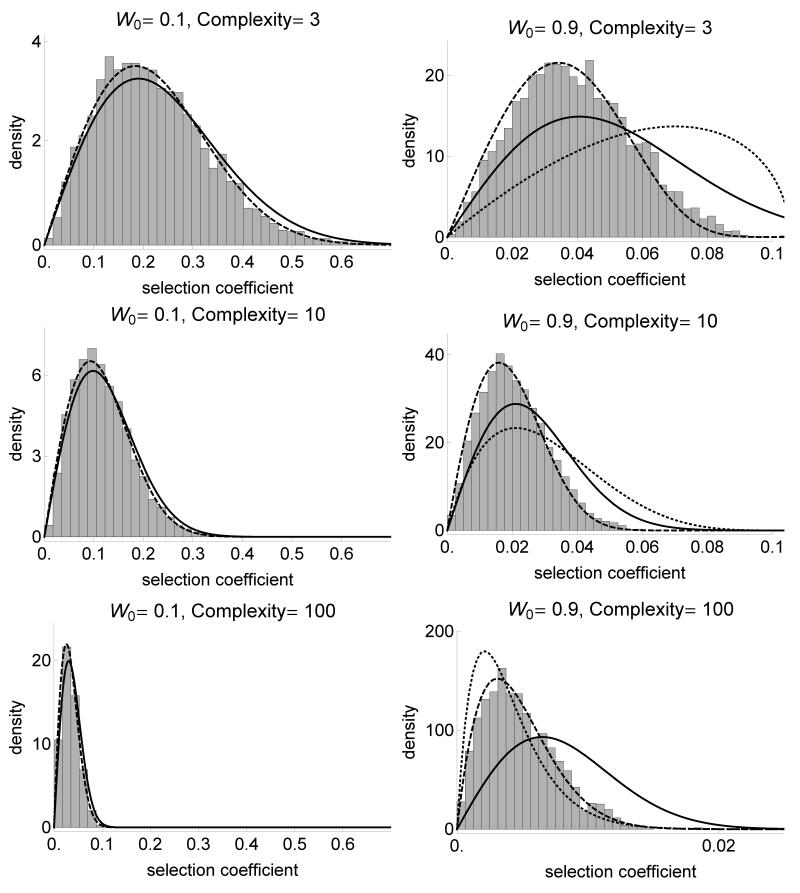
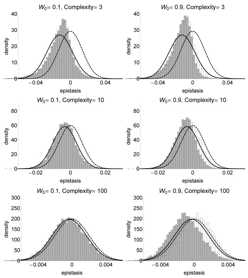
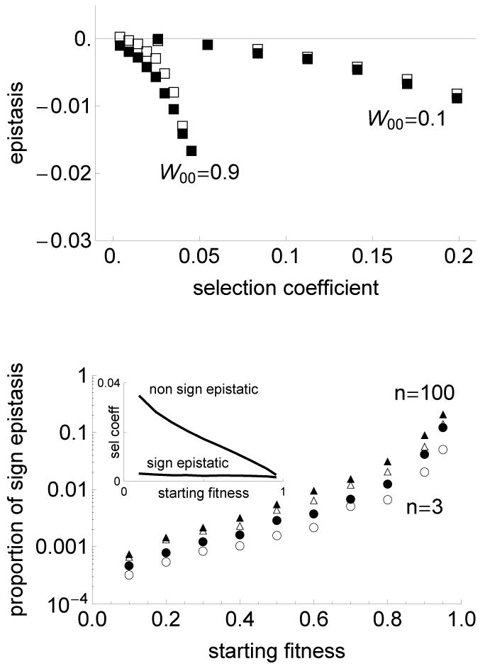
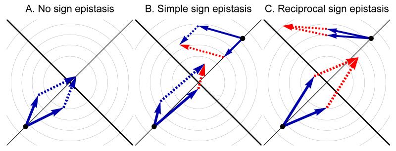
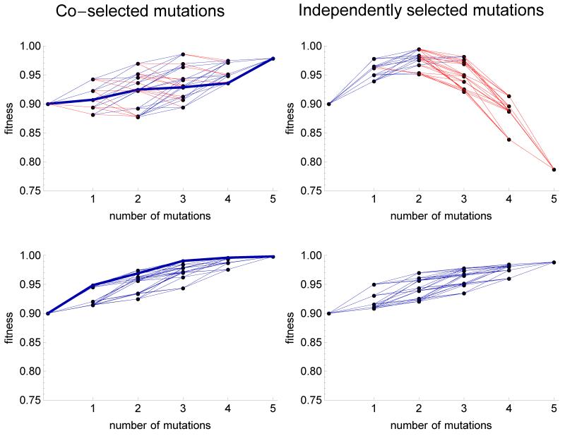
The fitness landscape-the mapping between genotypes and fitness-determines properties of the process of adaptation. Several small genotypic fitness landscapes have recently been built by selecting a handful of beneficial mutations and measuring fitness of all combinations of these mutations. Here, we generate several testable predictions for the properties of these small genotypic landscapes under Fisher's geometric model of adaptation. When the ancestral strain is far from the fitness optimum, we analytically compute the fitness effect of selected mutations and their epistatic interactions. Epistasis may be negative or positive on average depending on the distance of the ancestral genotype to the optimum and whether mutations were independently selected, or coselected in an adaptive walk. Simulations show that genotypic landscapes built from Fisher's model are very close to an additive landscape when the ancestral strain is far from the optimum. However, when it is close to the optimum, a large diversity of landscape with substantial roughness and sign epistasis emerged. Strikingly, small genotypic landscapes built from several replicate adaptive walks on the same underlying landscape were highly variable, suggesting that several realizations of small genotypic landscapes are needed to gain information about the underlying architecture of the fitness landscape.

Keywords: Adaptation; NK model; Rough Mount Fuji; epistasis; experimental evolution; selection.

Figure 1

The geometry of selected mutations in Fisher’s fitness landscape for various complexities of the phenotypic space. The left panel represents an isotropic landscape with n = 3. The log-fitness isocline in the phenotypic space is a sphere centered at the origin $\left(\log \right[W\left[z\right]]=-{\Sigma }_{i=1}^n{z}_i^2)$. The vertical axis is the main axis of selection. The ancestral strain and the optimum are shown as black points. A beneficial mutation is shown as a plain arrow. The geometry of the mutation is characterized by the norm ||z|| and by the angle between the mutations and the main axis of selection θ. On the right panel, the distribution of these quantities is shown for complexities n = 3, n = 10, n = 100. The mutational variance σ_mut was normalized such that the expected norm is the same for all complexities. At higher complexities, mutations tend to be almost orthogonal to the main axis of selection (θ → π/2) and to exhibit very little variation in their norm.

Figure 2

Distribution of the selection coefficient under Fisher’s model for various fitnesses of the ancestral strain W₀ (left: far from the optimum, right: near the optimum) and various complexities of the phenotypic space (from bottom to top). The line is the χ₂ analytical approximation (equation 2), the dashed line is based on the gamma approximation developed in Martin and Lenormand (2006) (Appendix) and the dotted line for W₀ = 0.9 is the beta approximation developed in Martin and Lenormand (2008). Selection coefficient is calculated for 10000 selected mutations. σ_mut is scaled such that the average norm of the mutational effect on phenotype is constant equal to 0.1 across complexities. The population size is N = 10⁷ and the mutation rate μ = 10⁻⁹.

Figure 3

Distribution of the epistasis coefficient e between two independently selected mutations (grey) and for co-selected mutations (white) for various fitnesses of the ancestral strain W₀ (left: far from the optimum, right: near the optimum) and complexities of the phenotypic space (from bottom to top). The plain line is the analytical approximation for independently selected mutations based on a normal distribution with mean and variance given by equation (4), and the dashed line is the normal approximation for random (newly arising) mutations (Martin et al. 2007). For independently selected mutations, the first mutations sweeping through the population in each of 20000 independent replicates were selected, and epistasis coefficient is calculated for 10000 independent pairs of selected mutations. For co-selected mutations, the first two mutations sweeping through the population in each of 10000 independent replicates were selected, resulting in 10000 independent epistasis coefficients. σ_mut is scaled such that the average norm of the mutational effect on phenotype is constant equal to 0.1 across complexities. The population size is N = 10⁷ and the mutation rate μ = 10⁻⁹.

Figure 4

Relationship between epistasis and the selection coefficient. Top panel: average epistasis coefficient between pairs of mutations as a function of the average selection coefficient of the two mutations, when W₀₀ = 0.1 and W₀₀ = 0.9, between independently selected mutations (filled squares) and co-selected mutations (open squares). For each parameter set, the selection coefficients were binned in 10 intervals of size (s_max − s_min)/10 and the average epistasis was computed for each of these bins when at least 10 pairs of mutations were present. For all curves complexity n = 10 (relationships are similar for other values of n). Bottom panel: Fraction of sign epistasis between two independently selected mutations (filled symbols) and between two co-selected mutations (open symbols). This is shown for complexities of the phenotypic space n = 3 (circles) and 100 (triangles). Inset shows the average coefficient of selection among non sign epistatic mutations (top curve) and sign epistatic mutations (bottom curve), as a function of the starting fitness, for complexity n = 3 and independently selected mutations (curves are similar for other parameters and selection procedure). The fraction of sign epistasis is calculated among at least 2000 independent pairs of mutations. Other parameters as in fig. 3.

Figure 5

The geometry of sign epistasis among two mutations in a two-dimensional Fisher’s fitness landscape model. The light gray lines are the fitness isoclines and the black lines are the phenotypic axes. Beneficial and deleterious mutations are shown respectively as blue and red arrows in the phenotypic space. In panel A, the two mutations are beneficial in the ancestral background and in the background with the other mutation (no sign epistasis). In panels B and C, two examples of pairs of sign epistatic mutations are shown. In B, one of the mutations is deleterious in the background with the other mutation (simple sign epistasis). In C, both mutations are deleterious in the background with the other mutation (reciprocal sign epistasis). In B and C, sign epistasis may occur by antagonistic pleiotropy (up, right) or optimum overshooting (bottom, left).

Figure 6

The distribution of the roughness to slope ratio and the fraction of sign epistasis over 1000 genotypic fitness landscapes generated with 5 mutations. Top left panel: distribution of roughness to slope ratio when W₀₀ = 0.1, for three levels of complexity, for independently selected mutations (distributions for co-selected mutations are very similar). In these conditions, there is no sign epistasis in more than 95% of the landscapes. Top right panel: distribution of the statistics in independently selected (blue) vs. co-selected mutations (purple). Bottom panel: distribution of the statistics for different levels of complexity (n = 3, n = 10, n = 100 in blue, red, green) in independently selected mutations (left) and co-selected mutations (right). Statistics corresponding to three experimental landscapes are superimposed (C: Chou et al. 2011, K: Khan et al. 2011, W: Weinreich et al. 2006).

Figure 7

Rough (top) and smooth (bottom) fitness landscapes obtained with 5 co-selected (left) or independently selected (right) mutations in Fisher’s model, with the same parameters (n = 3, W₀₀ = 0.9). Fitness of the 2⁵ = 32 genotypes is shown as a function of the number of mutations relative to the ancestor. The black points represent genotypes’ fitnesses, and the blue and red links are beneficial and deleterious mutations respectively. The thicker links represent the evolutionary path that was actually taken in the simulation, for co-selected mutations. In some cases, the genotypic landscape generated by independently selected mutations reflects quite clearly the presence of an optimum in fitness.

References

References of Appendix
1. Fisher R. The genetical theory of natural selection. Clarendon Press; 1930.
1. Kimura M. The neutral theory of molecular evolution. Cambridge University Press; Cambridge: 1983.
1. Lourenço J, Galtier N, Glémin S. Complexity, pleiotropy, and the fitness effect of mutations. Evolution. 2011;65(6):1559–1571. - PubMed
1. Martin G, Elena SF, Lenormand T. Distributions of epistasis in microbes fit predictions from a fitness landscape model. Nature genetics. 2007;39(4):555–560. - PubMed
1. Martin G, Lenormand T. A general multivariate extension of Fisher’s geometrical model and the distribution of mutation fitness effects across species. Evolution. 2006;60(5):893–907. - PubMed
1. Achaz G, Rodriguez-Verdugo A, Gaut BS, Tenaillon O. Ecological Genomics. Springer; 2014. The reproducibility of adaptation in the light of experimental evolution with whole genome sequencing; pp. 211–231. - PubMed
1. Bataillon T, Bailey SF. Effects of new mutations on fitness: insights from models and data. Annals of the New York Academy of Sciences. 2014;1320:76–92. - PMC - PubMed
1. Carneiro M, Hartl DL. Adaptive landscapes and protein evolution. Proceedings of the National Academy of Sciences. 2010;107(suppl 1):1747–1751. - PMC - PubMed
1. Chevin L-M, Decorzent G, Lenormand T. Niche dimensionality and the genetics of ecological speciation. Evolution. 2014;68(5):1244–1256. - PubMed
1. Chevin L, Martin G, Lenormand T. Fisher’s model and the genomics of adaptation: restricted pleiotropy, heterogeneous mutation, and parallel evolution. Evolution. 2010;64(11):3213–3231. - PubMed
Publication types