. 2014 Oct 6;22(20):24411-29.
doi: 10.1364/OE.22.024411.

Quantitative technique for robust and noise-tolerant speed measurements based on speckle decorrelation in optical coherence tomography

Quantitative technique for robust and noise-tolerant speed measurements based on speckle decorrelation in optical coherence tomography

Néstor Uribe-Patarroyo et al. Opt Express. .

Abstract

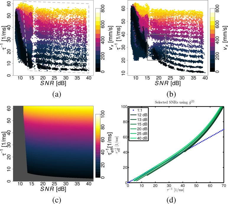
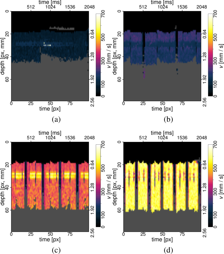
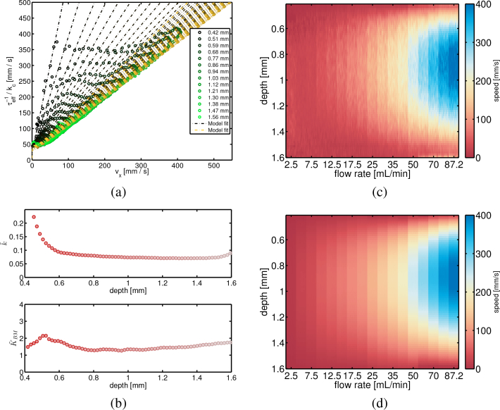
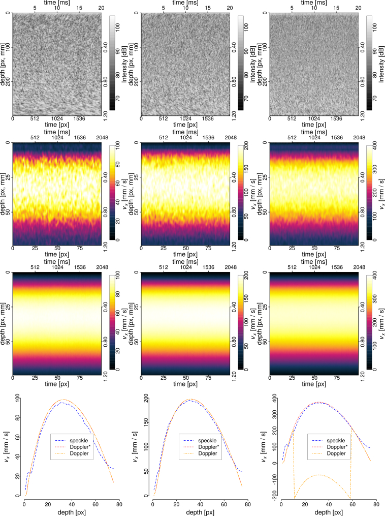
Intensity-based techniques in optical coherence tomography (OCT), such as those based on speckle decorrelation, have attracted great interest for biomedical and industrial applications requiring speed or flow information. In this work we present a rigorous analysis of the effects of noise on speckle decorrelation, demonstrate that these effects frustrate accurate speed quantitation, and propose new techniques that achieve quantitative and repeatable measurements. First, we derive the effect of background noise on the speckle autocorrelation function, finding two detrimental effects of noise. We propose a new autocorrelation function that is immune to the main effect of background noise and permits quantitative measurements at high and moderate signal-to-noise ratios. At the same time, this autocorrelation function is able to provide motion contrast information that accurately identifies areas with movement, similar to speckle variance techniques. In order to extend the SNR range, we quantify and model the second effect of background noise on the autocorrelation function through a calibration. By obtaining an explicit expression for the decorrelation time as a function of speed and diffusion, we show how to use our autocorrelation function and noise calibration to measure a flowing liquid. We obtain accurate results, which are validated by Doppler OCT, and demonstrate a very high dynamic range (> 600 mm/s) compared to that of Doppler OCT (±25 mm/s). We also derive the behavior for low flows, and show that there is an inherent non-linearity in speed measurements in the presence of diffusion due to statistical fluctuations of speckle. Our technique allows quantitative and robust measurements of speeds using OCT, and this work delimits precisely the conditions in which it is accurate.


Figures

Fig. 1
Fig. 1
Measurement setup. The xyz coordinate system was defined by the light propagation direction z and its associated perpendicular plane xy (y towards the reader). The solid rubber phantom traveled in the x direction on a motorized linear stage. Inset: configuration for measuring signals from flowing intralipid. The beam was reflected almost perpendicular to the fiber after internal reflection (a rotation around y). The angle between the beam and the flow was θ = 82.5°.
Fig. 2
Fig. 2
(left) M-mode tomogram of phantom fluid at 2.5 mL/min with low flow velocities and large horizontal speckle size, (right) the same sample at 80 mL/min yielding high flow speeds and small horizontal speckle size. The strong reflections at the top correspond to the lens and other surfaces of the probe, the wall of the tube is the weak reflection at the bottom. The depth scale in mm is approximate as the index of refraction of the different materials has been considered equal to the fluid’s index 1.33.
Fig. 3
Fig. 3
(a–b) Mean intensity of the structural image, (c–d) inverse correlation time profiles for moving solid sample using the traditional autocorrelation function and (e–f) using the newly developed normalized autocorrelation function. (g–h) Profile comparing the inverse decorrelation time using the new and the traditional autocorrelation function at a selected column. Top row corresponds to 120 mm/s, bottom row to 240 mm/s.
Fig. 4
Fig. 4
(top) Traditional autocorrelation at selected depths for the solid sample moving at (left) 120 mm/s, (center) 200 mm/s and (right) 400 mm/s. The autocorrelation for 20 px at 400 mm/s is out of the range. (bottom) The new normalized autocorrelation for the same speeds.
Fig. 5
Fig. 5
(a) Scatter plot of τ−1 and SNR for different sample speeds as calculated using Eq. (18). (b) Scatter plot of the same data using the Pearson autocorrelation function. (c) Parametrization F of the effective inverse correlation time as a function of inverse correlation time and SNR, Eq. (23). (d) τeff1 as a function of τ−1 in the parametrization for several representative SNRs. Note the undefined value for low SNRs and low τ−1, as well as a unity slope line 1 : 1 as a visual guide.
Fig. 6
Fig. 6
Speed profiles for moving solid sample using τeff1. (a) 40 mm/s, (b) 100 mm/s, (c) 200 mm/s and (d) 300 mm/s. The areas in dark gray that denote where it is not possible to uniquely determine the speed due to the low SNR.
Fig. 7
Fig. 7
(a) Scatter plot of the time-averaged effective inverse speckle-decorrelation time τeff and the measured Doppler velocity vx for different data sets in the liquid setup. The colors denote the depth, from black to green (yellow) for the experimental data (model fit). (b) Fitting parameters as a function of depth. (c) Flow speed as determined by speckle correlation of the calibration dataset. Each flow rate has 50 flow profiles in time, and all flow rates are shown in sequence. (d) Reference Doppler velocity of the calibration dataset.
Fig. 8
Fig. 8
Structural image of the first 2048 A-lines (first row), speckle decorrelation flow speed (second row), line-of-sight-corrected Doppler flow speed (third row) and time-average flow speed profiles (fourth row) for intralipid solution at 20 mL/min, 40 mL/min, and 80 mL/min flow rates in 3.2 mm-diameter tubing. The depth is measured from the surface of the sheath, which has a 0.4 mm radius. Doppler* indicates the signal after unwrapping.

Similar articles

Cited by

References

    1. Bouma B. E., Tearney G. J., eds., Handbook of optical coherence tomography (Marcel Dekker Inc, 2002).
    1. Yonetsu T., Bouma B. E., Kato K., Fujimoto J. G., Jang I.-K., “Optical coherence tomography,” Circulation J. 77, 1933–1940 (2013).10.1253/circj.CJ-13-0643.1 - DOI - PubMed
    1. Wiesauer K., Pircher M., Götzinger E., Bauer S., Engelke R., Ahrens G., Grützner G., Hitzenberger C., Stifter D., “En-face scanning optical coherence tomography with ultra-high resolution for material investigation,” Opt. Express 13, 1015–1024 (2005).10.1364/OPEX.13.001015 - DOI - PubMed
    1. Wiesauer K., Pircher M., Goetzinger E., Hitzenberger C. K., Engelke R., Ahrens G., Gruetzner G., Stifter D., “Transversal ultrahigh-resolution polarizationsensitive optical coherence tomography for strain mapping in materials,” Opt. Express 14, 5945–5953 (2006).10.1364/OE.14.005945 - DOI - PubMed
    1. Stifter D., Leiss-Holzinger E., Major Z., Baumann B., Pircher M., Götzinger E., Hitzenberger C. K., Heise B., “Dynamic optical studies in materials testing with spectral-domain polarization-sensitive optical coherence tomography,” Opt. Express 18, 25712–25725 (2010).10.1364/OE.18.025712 - DOI - PubMed

Publication types

LinkOut - more resources