The cellular origins of the outer retinal bands in optical coherence tomography images

Abstract

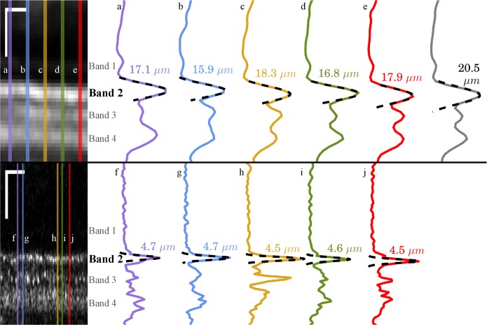
Purpose: To test the recently proposed hypothesis that the second outer retinal band, observed in clinical OCT images, originates from the inner segment ellipsoid, by measuring: (1) the thickness of this band within single cone photoreceptors, and (2) its respective distance from the putative external limiting membrane (band 1) and cone outer segment tips (band 3).

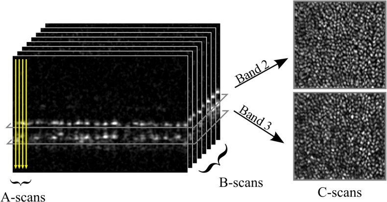
Methods: Adaptive optics-optical coherence tomography images were acquired from four subjects without known retinal disease. Images were obtained at foveal (2°) and perifoveal (5°) locations. Cone photoreceptors (n = 9593) were identified and segmented in three dimensions using custom software. Features corresponding to bands 1, 2, and 3 were automatically identified. The thickness of band 2 was assessed in each cell by fitting the longitudinal reflectance profile of the band with a Gaussian function. Distances between bands 1 and 2, and between 2 and 3, respectively, were also measured in each cell. Two independent calibration techniques were employed to determine the depth scale (physical length per pixel) of the imaging system.

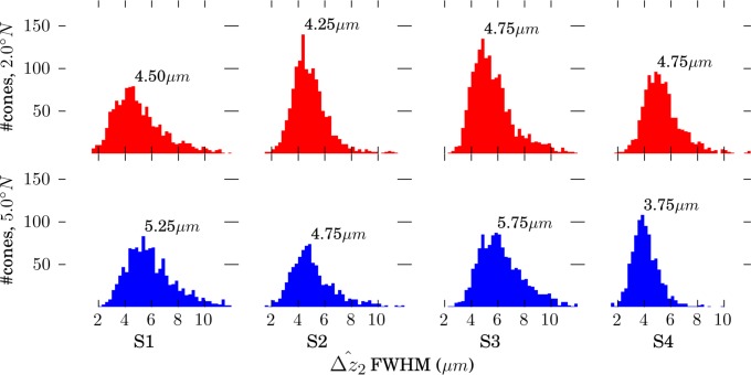
Results: When resolved within single cells, the thickness of band 2 is a factor of three to four times narrower than in corresponding clinical OCT images. The distribution of band 2 thickness across subjects and eccentricities had a modal value of 4.7 μm, with 48% of the cones falling between 4.1 and 5.2 μm. No significant differences were found between cells in the fovea and perifovea. The distance separating bands 1 and 2 was found to be larger than the distance between bands 2 and 3, across subjects and eccentricities, with a significantly larger difference at 5° than 2°.

Conclusions: On the basis of these findings, we suggest that ascription of the outer retinal band 2 to the inner segment ellipsoid is unjustified, because the ellipsoid is both too thick and proximally located to produce the band.

Keywords: adaptive optics; morphometry; nomenclature; optical coherence tomography; photoreceptor morphology.

Figure 1

Comparison of conventional OCT with AO-OCT. Horizontal wide-field Spectralis B-scan centered on the fovea of one of the study's subjects (left). Image is displayed as the instrument displays it, in logarithmic scale. Red and blue boxes indicate locations, 2.0° nasal and 5.0° nasal, used for AO-OCT imaging. Magnified view (near right) of a portion of the Spectralis image containing outer retinal layers at 5.0° nasal, in linear scale. Corresponding AO-OCT image (far right) from the same location in the same subject, also shown in linear scale. In both inset images, the outer retinal layers 1 through 4 are labeled. Bands 1, 3, and 4 correspond to putative ELM, COST, and RPE, respectively. The controversy surrounding the origin of band 2 is the subject of the present investigation. For the Spectralis, linearizing required use of the instrument's reported dynamic range (43 dB). All of the qualitative and quantitative observations presented in this paper were performed using linear intensity for both Spectralis and AO-OCT images. The Spectralis was operated in ‘ART' mode, and the resulting image is an average of 100 frames. The AO-OCT image shown is a single frame. In magnified views, scale bars (white) indicate 50 μm in lateral and axial dimensions.

Figure 2

In SD-OCT, a point source is scanned over the retina, acquiring one axial scan (A-scan) per retinal location. If the point source is scanned in a line across the retina, a 2D, cross-sectional image of the retina (B-scan) is created. If the point source is raster scanned, in two dimensions, a 3D, volumetric image may be generated. From the latter, areal (or en face) projections of the retinal layers at specific depths (C-scans) may be extracted. C-scans from the depths of bands 2 and 3 are shown (right). Both reveal regular mosaics of the overlapping bright spots whose spacing agrees with histologic measurements of cone photoreceptors. At both layers, reflected light appears to be confined, laterally, to the interior of the cell.

Figure 3

Typical areal projection of band 2, from S3 at 5°, the same portion of retina shown in Figure 4. The full mosaic is shown on the left, and the cones automatically identified and segmented for analysis on the right. A number of cones were clearly missed by the algorithm, which was intentionally tuned to favor a low false-positive rate over a low miss rate. In spite of the misses, more than a thousand cones were found, on average, in a volumetric image. Scale bars: 50 μm.

Figure 4

Topography (in μm) of band 2, from S3 at 5°, the same portion of retina shown in Figures 3 and 5. Our custom model-based classification algorithm located the depth of band 2 in the retina automatically (see Appendix). The resulting topography (left) revealed a wide spectrum of height variation. Low frequency variation was due to gross curvature of the retina and axial eye movements. High frequency variation was due to axial displacements among neighboring cone cells, which are more evident after high-pass filtering the topographic image (right). The boxes denote areas with numerous segmentation errors. Those in the black box fall under an intervening blood vessel (visible in Fig. 3), and result from the relatively low reflectance of the underlying cones. Those in the green box are due to a 20-μm region in which cone visibility is poor for an unknown reason (also visible in Fig. 3). Roughness of the high-pass filtered surface was quantified by computing the depth variance along fast scans in the corrected image and taking the square root of the average of those variances. The resulting roughness was 1.6 ± 0.3 μm. Scale bars: 50 μm.

Figure 5

Band thickness measured with Spectralis OCT and AO-OCT. A 210-μm wide section of a Spectralis B-scan (top left), acquired from S3 at 5.0° and converted to linear intensity scale. The Spectralis instrument permits saving of log-intensity data only; in order to convert to a linear scale, the system's reported dynamic range (43 dB) was used. The overlaid lines indicate the locations of the five A-scans plotted at (top right), labeled a-e. The sixth (gray) plot represents the average of 10 A-scans (56 μm), equal to the size of regions analyzed by other investigators. Overlaid on each plot is a least-squares Gaussian fit (dashed line), from which the FWHM of the peak can be readily calculated, indicated for each plotted A-scan. A comparable AO-OCT B-scan (bottom left) from the same subject and eccentricity, also shown in linear scale. Locations for the plotted A-scans (bottom right), labeled f-j, were selected by identifying bright cones in the image. Full-width half maximum values, calculated the same way, were considerably smaller. Note that in both OCT and AO-OCT, averaging over multiple cells leads to an overestimate of layer thickness, due to axial displacements of the reflections. Scale bars: 50 μm.

Figure 6

Distributions of band 2 thickness in four subjects, measured at two retinal eccentricities. Each distribution was binned at 0.25-μm intervals, and mode (fullest bin) thickness is shown for each plot. Mean thickness was 0.5 to 1.5-μm larger than the mode.

Figure 7

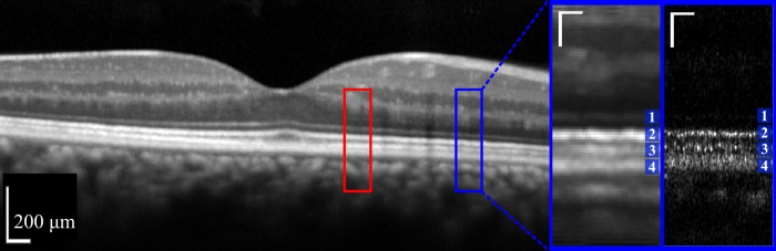
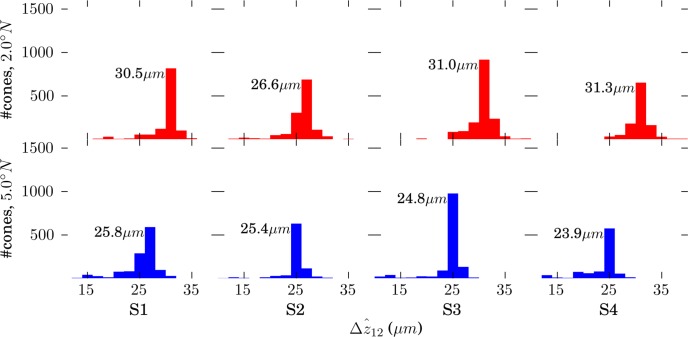
Distributions of , defined by the distance between peak of the band 1 (ELM) reflection and the peak of the band 2 reflection. Because no subpixel fitting of peaks was employed, precision was limited by the 0.74 μm (RMS) axial quantization error.

Figure 8

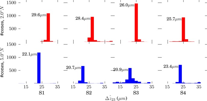
Distributions of , defined by the distance between peak of the band 2 reflection and the peak of the band 3 reflection. Because no subpixel fitting of peaks was employed, precision was limited by the 0.74 μm (RMS) axial quantization error.

Figure 9

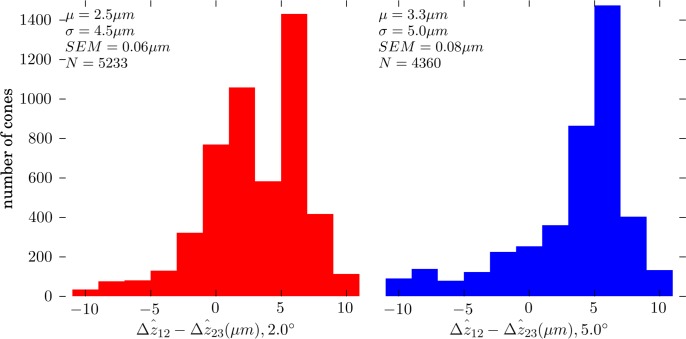
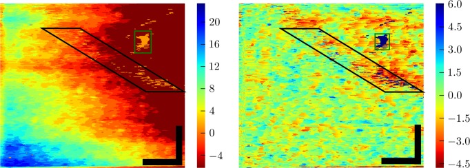
Distributions of at 2.0° (left) and 5.0° (right), for all four subjects. At both eccentricities for most cones, with average differentials of + 2.5 and + 3.3 μm at 2.0° and 5.0°, respectively. Thus, band 2 lies approximately between band 1 (ELM) and band 3, but slightly closer to the latter.

Figure 10

An electron micrograph of a partial human cone photoreceptor (reprinted with permission from Hogan MJ, Alvarado JA, Weddell JE. Histology of the Human Eye: An Atlas and Textbook. Philadelphia: Saunders; 1971. Copyright Elsevier; annotations modified). The image shows portions of the cone IS (top) and OS (bottom). The portion of IS shown is a part of the IS ellipsoid (ISe), densely packed with mitochondria (each ~3-μm long), arranged with their long axes parallel to the optical axis of the cone. In the OS, the stacked discs (~50-nm spacing) are clearly visible. Only a small portion of the ISe and OS fall within the micrograph; at this scale, the segments would each span the entirety of this page. Also visible is the distal membrane of the IS, seen here (and in comparable micrographs from other sources, see text) to lie at an angle to the cell's optical axis. The newest 10 to 15 discs, at the proximal edge of the OS, are narrower than mature discs. The slope of the distal IS membrane is similar to the slope of the proximal edge of the OS. In this image, and others like it, a narrow (50–200 nm) gap is visible between the distal IS membrane and proximal discs of the OS (yellow arrow). It is not known whether this gap is an artifact of tissue preparation for electron microscopy or whether it corresponds to a region of interstitial fluid that separates the IS and OS.

References

1. Gabriele ML, Wollstein G, Ishikawa H, et al. Three dimensional optical coherence tomography imaging: advantages and advances. Prog Retin Eye Res. 2010; 29: 556–579. - PMC - PubMed
1. Huang D, Swanson EA, Lin CP, et al. Optical coherence tomography. Science. 1991; 254: 1178–1181. - PMC - PubMed
1. Schuman JS, Hee MR, Puliafito CA, et al. Quantification of nerve fiber layer thickness in normal and glaucomatous eyes using optical coherence tomography. Arch Ophthalmol. 1995; 113: 586–596. - PubMed
1. Blumenthal EZ, Williams JM, Weinreb RN, Girkin CA, Berry CC, Zangwill LM. Reproducibility of nerve fiber layer thickness measurements by use of optical coherence tomography. Ophthalmology. 2000; 107: 2278–2282. - PubMed
1. Guedes V, Schuman JS, Hertzmark E, et al. Optical coherence tomography measurement of macular and nerve fiber layer thickness in normal and glaucomatous human eyes. Ophthalmology. 2003; 110: 177–189. - PMC - PubMed