Random-effects, fixed-effects and the within-between specification for clustered data in observational health studies: a simulation study

Abstract

Background: When unaccounted-for group-level characteristics affect an outcome variable, traditional linear regression is inefficient and can be biased. The random- and fixed-effects estimators (RE and FE, respectively) are two competing methods that address these problems. While each estimator controls for otherwise unaccounted-for effects, the two estimators require different assumptions. Health researchers tend to favor RE estimation, while researchers from some other disciplines tend to favor FE estimation. In addition to RE and FE, an alternative method called within-between (WB) was suggested by Mundlak in 1978, although is utilized infrequently.

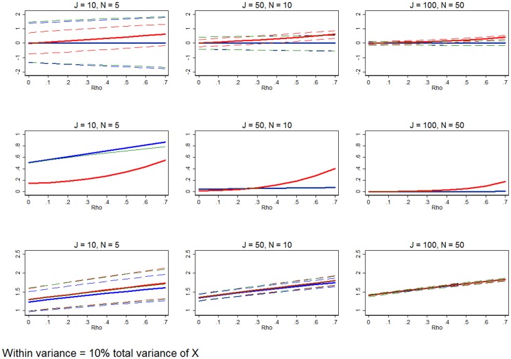
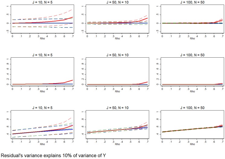
Methods: We conduct a simulation study to compare RE, FE, and WB estimation across 16,200 scenarios. The scenarios vary in the number of groups, the size of the groups, within-group variation, goodness-of-fit of the model, and the degree to which the model is correctly specified. Estimator preference is determined by lowest mean squared error of the estimated marginal effect and root mean squared error of fitted values.

Results: Although there are scenarios when each estimator is most appropriate, the cases in which traditional RE estimation is preferred are less common. In finite samples, the WB approach outperforms both traditional estimators. The Hausman test guides the practitioner to the estimator with the smallest absolute error only 61% of the time, and in many sample sizes simply applying the WB approach produces smaller absolute errors than following the suggestion of the test.

Conclusions: Specification and estimation should be carefully considered and ultimately guided by the objective of the analysis and characteristics of the data. The WB approach has been underutilized, particularly for inference on marginal effects in small samples. Blindly applying any estimator can lead to bias, inefficiency, and flawed inference.

Figure 1. Prevalence of random- and fixed-effects in health, economics, and political science literature.

Each archive was searched for the terms “random effects” or “random effect” and “fixed effects” or “fixed effect” present in abstracts. Papers that also used the term “meta” in the abstract were not included in to avoid including meta-analyses which is a very specific use of RE and FE estimation. PubMed is a database that archives life science and biomedical abstracts and references, primarily drawn from the MEDLINE database. EconLit is also an archiving database, published by the American Economic Association, which focuses on economics literature. PAIS is the Public Affairs Information Service International database, which archives references focusing on public affairs.

Figure 2. Distribution of errors.

Red lines show the distribution of errors from RE estimation, while the blue lines show the distribution of errors from FE estimation. Each panel shows the correlation between the explanatory variable and the group-level effect set to a different value of ρ (0.0, 0.3, 0.6), increasing from left to right. Simulation based on the correct specification of a model with 50 groups and 10 observations per group. 50% of the variation of the outcome variable is explained by residuals, while only 10% of the variation in the explanatory variable is within-groups.

Figure 3. Distribution of errors of estimated marginal effects at baseline specification.

The solid red line shows the mean error in the marginal effect estimates from RE estimation, while the dashed red lines show the 95% range of the RE estimation errors. The solid blue line and dashed blue lines show that mean and 95% range of the errors from FE estimation. The solid green line and dashed green lines show that mean and 95% range of the errors from the WB approach. All simulation inputs are baseline.

Figure 4. MSE of marginal effect estimates at baseline.

The red line shows the MSE from the errors in the marginal effect estimates from RE estimation. The blue and green lines shows the same for FE estimation and WB approach, respectively. All simulation inputs are baseline.

Figure 5. Hausman test.

The solid orange lines show the share of the simulations for which the Hausman test does not reject, at the 90% confidence level, the null hypothesis that both RE and FE estimation are consistent. Conventional wisdom is that this suggests that researchers should use RE estimation as it is more efficient. The dashed orange lines show the share of the simulations for which the Hausman test suggests the estimator with smaller absolute error. The red background indicates when the RE estimator is MSE-preferred, while the blue background indicates when the FE estimator is MSE-preferred. The white regions indicate that the difference between the MSE of the two estimators is trivial. All simulation inputs are baseline.

Figure 6. Distribution of RMSE from predicted outcomes.

The red lines show the mean and 95% confidence interval of the RMSE derived from the fitted values using RE estimation. Each combination of inputs is made up of 1,000 simulations, and each receives its own RMSE based on the errors of the fitted values. The blue lines show the mean and 95% range of the RMSE acquired using the FE estimator. The green lines show the mean and 95% range of the RMSE from the WB approach. All simulation inputs are baseline.

Figure 7. Significant between-group variation relative to within-group variation.

Row 1 (interpreted like Figure 3) shows the distribution of the errors in marginal effects estimates from the RE estimation (red), FE estimation (blue), and WB approach (green). Row 2 (interpreted like Figure 4) shows MSE associated with the RE estimation (red), FE estimation (blue), and WB approach (green) errors. Row 3 (interpreted like Figure 6) shows the distribution of the RMSE from the fitted values estimated using RE estimation (red), FE estimation (blue), and WB approach (green). The between-group variation is set to 0.9, while the within-group variation is 0.1. All other simulation input parameters are set to baseline.

Figure 8. Significant within-group variation relative to between-group variation.

Row 1 (interpreted like Figure 3) shows the distribution of the errors in marginal effects estimates from the RE estimation (red), FE estimation (blue), and WB approach (green). Row 2 (interpreted like Figure 4) shows MSE associated with the RE estimation (red), FE estimation (blue), and WB approach (green) errors. Row 3 (interpreted like Figure 6) shows the distribution of the RMSE from the fitted values estimated using RE estimation (red), FE estimation (blue), and WB approach (green). The within-group variation is set to 0.75, while the between-group variation is 0.25. All other simulation input parameters are set to baseline.

Figure 9. Poorly fit model that explains only a small portion of the outcome variable's variance.

Row 1 (interpreted like Figure 3) shows the distribution of the errors in marginal effects estimates from the RE estimation (red), FE estimation (blue), and WB approach (green). Row 2 (interpreted like Figure 4) shows MSE associated with the RE estimation (red), FE estimation (blue), and WB approach (green) errors. Row 3 (interpreted like Figure 6) shows the distribution of the RMSE from the fitted values estimated using RE estimation (red), FE estimation (blue), and WB approach (green). The variance of the residual is set such that it explains 90% of the variation of the outcome variable. All other simulation input parameters are set to baseline.

Figure 10. Well fit model that explains a significant portion of the outcome variable's variance.

Row 1 (interpreted like Figure 3) shows the distribution of the errors in marginal effects estimates from the RE estimation (red), FE estimation (blue), and WB approach (green). Row 2 (interpreted like Figure 4) shows MSE associated with the RE estimation (red), FE estimation (blue), and WB approach (green) errors. Row 3 (interpreted like Figure 6) shows the distribution of the RMSE from the fitted values estimated using RE estimation (red), FE estimation (blue), and WB approach (green). The variance of the residual is set such that it explains only 10% of the variation of the outcome variable. All other simulation input parameters are set to baseline.

Figure 11. Misspecified model.

Row 1 (interpreted like Figure 3) shows the distribution of the errors in marginal effects estimates from the RE estimation (red), FE estimation (blue), and WB approach (green). Row 2 (interpreted like Figure 4) shows MSE associated with the RE estimation (red), FE estimation (blue), and WB approach (green) errors. Row 3 (interpreted like Figure 6) shows the distribution of the RMSE from the fitted values estimated using RE estimation (red), FE estimation (blue), and WB approach (green). The correlation between the explanatory variable and the residual is set to 0.2. All other simulation input parameters are set to baseline.

References

1. Kennedy P (2003) A Guide to Econometrics. 5th ed. Cambridge: The MIT Press. 500 p.
1. Schempf AH, Kaufman JS (2012) Accounting for context in studies of health inequalities: a review and comparison of analytic approaches. Ann Epidemiol 22: 683–690. - PubMed
1. Duncan C, Jones K, Moon G (1998) Context, Composition and Heterogeneity: Using Multilevel Models in Health Research. Soc Sci Med 46 (1): 97–117. - PubMed
1. Diez Roux AV (2002) A glossary for multilevel analysis. J Epidemiol Community Health 56: 588–594. - PMC - PubMed
1. Bingenheimer JB, Raudenbush SW (2004) Statistical and Substantive Inferences in Public Health: Issues in the Application of Multilevel Models. Annu Rev Public Health 25: 53–77. - PubMed
Publication types
LinkOut - more resources