Distal transport of dissolved hydrothermal iron in the deep South Pacific Ocean

Abstract

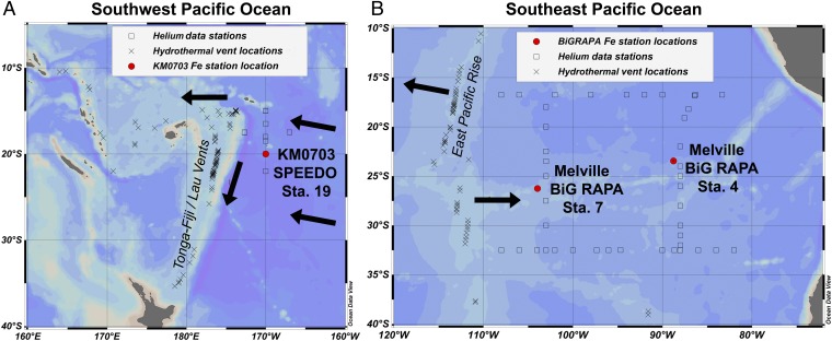
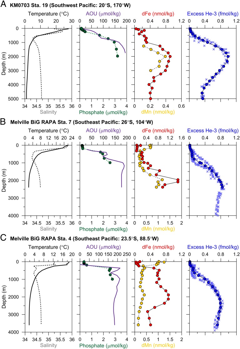
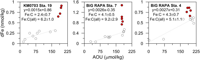
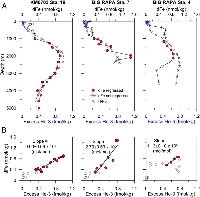
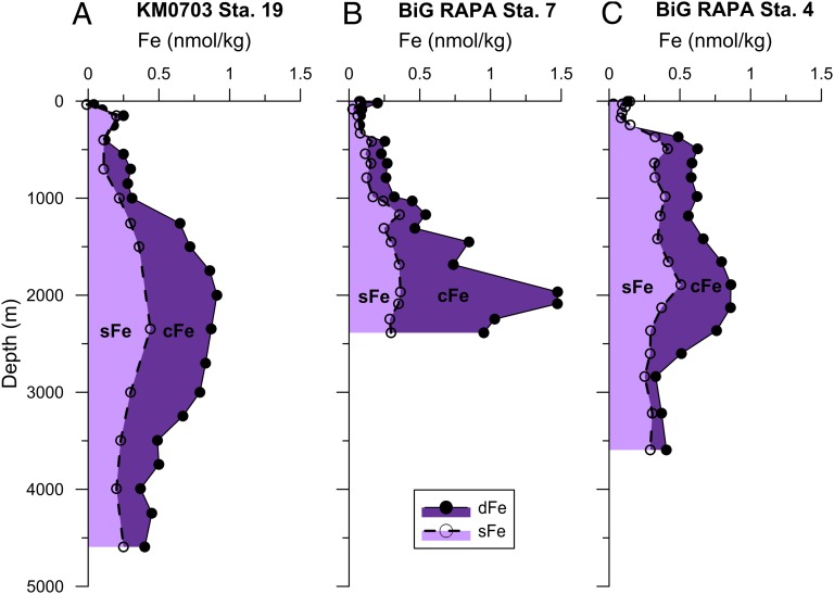
Until recently, hydrothermal vents were not considered to be an important source to the marine dissolved Fe (dFe) inventory because hydrothermal Fe was believed to precipitate quantitatively near the vent site. Based on recent abyssal dFe enrichments near hydrothermal vents, however, the leaky vent hypothesis [Toner BM, et al. (2012) Oceanography 25(1):209-212] argues that some hydrothermal Fe persists in the dissolved phase and contributes a significant flux of dFe to the global ocean. We show here the first, to our knowledge, dFe (<0.4 µm) measurements from the abyssal southeast and southwest Pacific Ocean, where dFe of 1.0-1.5 nmol/kg near 2,000 m depth (0.4-0.9 nmol/kg above typical deep-sea dFe concentrations) was determined to be hydrothermally derived based on its correlation with primordial (3)He and dissolved Mn (dFe:(3)He of 0.9-2.7 × 10(6)). Given the known sites of hydrothermal venting in these regions, this dFe must have been transported thousands of kilometers away from its vent site to reach our sampling stations. Additionally, changes in the size partitioning of the hydrothermal dFe between soluble (<0.02 µm) and colloidal (0.02-0.4 µm) phases with increasing distance from the vents indicate that dFe transformations continue to occur far from the vent source. This study confirms that although the southern East Pacific Rise only leaks 0.02-1% of total Fe vented into the abyssal Pacific, this dFe persists thousands of kilometers away from the vent source with sufficient magnitude that hydrothermal vents can have far-field effects on global dFe distributions and inventories (≥3% of global aerosol dFe input).

Keywords: East Pacific Rise; helium; hydrothermal vents; iron; trace metals.

Fig. 1.

Map of study locations. (A) The southwest Pacific, where KM0703 SPEEDO Station 19 (20°S, 170°W) is indicated in red and the hydrothermally active Tonga–Kermadec Arc is indicated as a topographic high along 175°W. (B) The southeast Pacific, where Melville BiG RAPA Stations 7 (26.25°S, 104°W) and 4 (23.5°S, 88.75°W) are indicated in red and the hydrothermally active EPR is designated. Shown as squares are stations of historical ³He data that were used to interpolate the average ³He profiles onto this study's sampling locations (historic ³He data from cchdo.ucsd.edu); the more proximal stations had a greater influence on the interpolated ³He profile than the distal stations. Shown as crosses are sites of confirmed or inferred hydrothermal venting deeper than 1,000 m (33). Directions of mean advection at 2,000 m (36) are indicated with black arrows.

Fig. 2.

Oceanographic profiles showing a hydrothermal influence on dFe, ³He, and dMn at 2,000 m. Relevant profiles taken from (A) SPEEDO-KM0703 Station 19 in the southwest Pacific, (B) Melville BiG RAPA Station 7 in the southeast Pacific, and (C) Melville BiG RAPA Station 4 in the southeast Pacific. Note that dFe SDs on replicate analyses (tabulated in Table S1) were typically the size of the symbol and are thus not shown. The interpolated excess ³He data are shown as blue circles at the depths where dFe measurements were made, whereas the data used to generate those average values are shown as light blue crosses.

Fig. 3.

dFe–AOU relationships for each of the three sampling locations: (Left) SPEEDO-KM0703 Station 19 in the southwest Pacific, (Middle) Melville BiG RAPA Station 7 in the southeast Pacific, and (Right) Melville BiG RAPA Station 4 in the southeast Pacific. The stations included in the Fe:C regression calculation are in open circles (∼500–1,000 m depth), whereas the red circles show the deeper sample depths affected by hydrothermal Fe; these correspond to the equivalent symbols in Fig. 4. The Fe:C ratio is derived from the regression (open circles only), whereas the ratio indicated as “Fe:C (all)” includes all points (even those experiencing hydrothermal Fe inputs in red). Fe:C ratios are calculated using an AOU:C ratio of 1.6 (61) and are in units of µmol/mol.

Fig. 4.

Distal hydrothermal dFe/³He. (A) dFe and ³He data and (B) the Type II regressions used to evolve dFe/³He ratios. Station locations are (Left) KM0703 Station 19 in the southwest Pacific, (Middle) BiG RAPA Station 7 in the southeast Pacific, and (Right) BiG RAPA Station 4 in the southeast Pacific. Data excluded from the dFe/³He regression calculation are shown in both A and B as open circles and include all data shallower than 1,000 m and the deepest samples of Stations 4 and 7, where dFe appears to have been scavenged, while ³He remains elevated.

Fig. 5.

The size partitioning of dFe into soluble and colloidal phases demonstrates continued Fe transformations at great distance from vents. Dissolved Fe (closed circles, solid line; dFe < 0.4 µm) is partitioned into soluble Fe (open circles, dashed line, light purple shading; sFe < 0.02 µm or 10 kDa) and colloidal Fe (cFe, the difference between the two lines in dark purple shading) fractions at (A) Station 19 in the southwest Pacific, (B) Station 7 in the southeast Pacific, and (C) Station 4 in the southeast Pacific. SDs are typically the size of the symbol and are thus not shown.

References

1. Moore JK, Doney SC, Glover DM, Fung IY. Iron cycling and nutrient-limitation patterns in surface waters of the World Ocean. Deep Sea Res Part II Top Stud Oceanogr. 2002;49(1-3):463–507.
1. Boyd PW, et al. Mesoscale iron enrichment experiments 1993-2005: Synthesis and future directions. Science. 2007;315(5812):612–617. - PubMed
1. Martin JH. Glacial-interglacial CO2 change: The iron hypothesis. Paleoceanography. 1990;5(1):1–13.
1. Moore JK, Doney SC, Lindsay K. Upper ocean ecosystem dynamics and iron cycling in a global three-dimensional model. Global Biogeochem Cycles. 2004;18(4):GB4028.
1. Von Damm KL, et al. Chemistry of submarine hydrothermal solutions at 21°N, East Pacific Rise. Geochim Cosmochim Acta. 1985;49(11):2197–2220.
Publication types
LinkOut - more resources