Stimulus dependence of local field potential spectra: experiment versus theory

Abstract

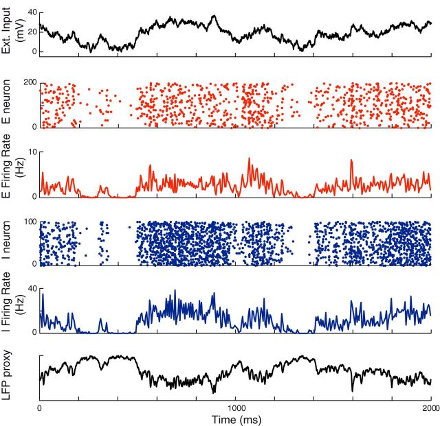
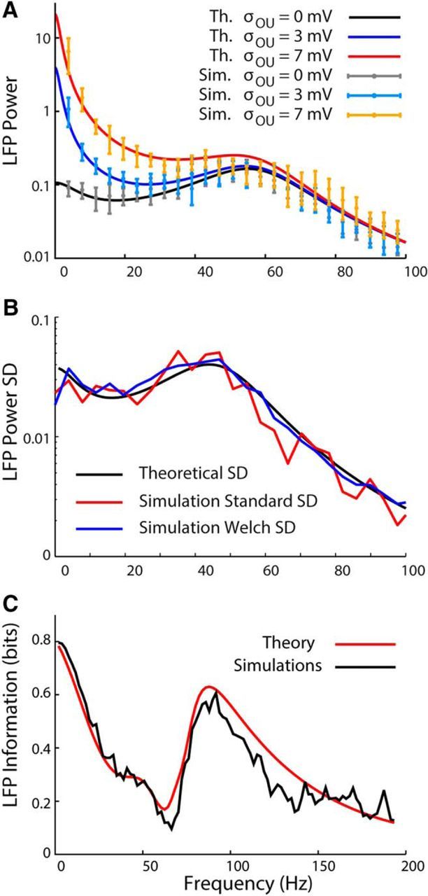
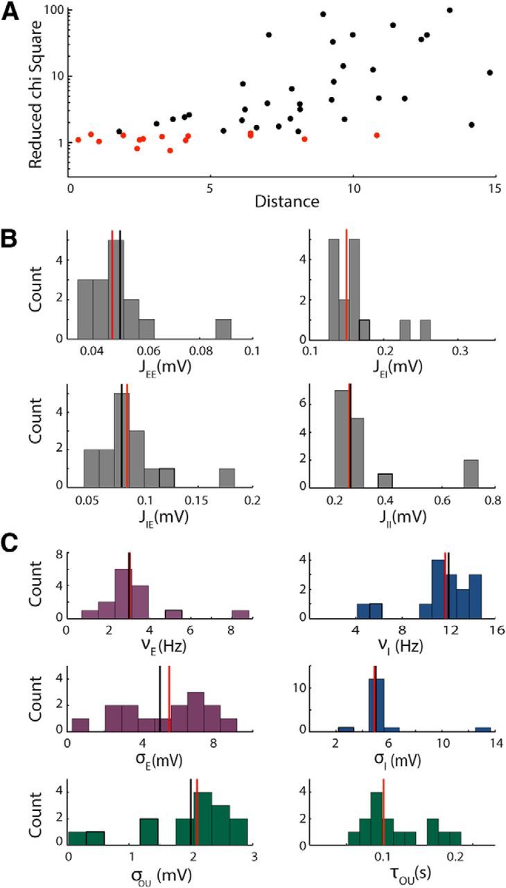
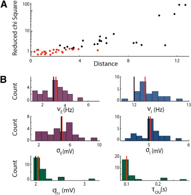
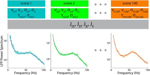
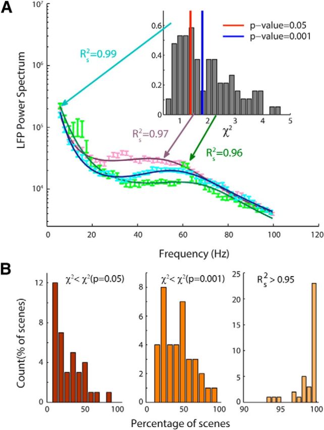
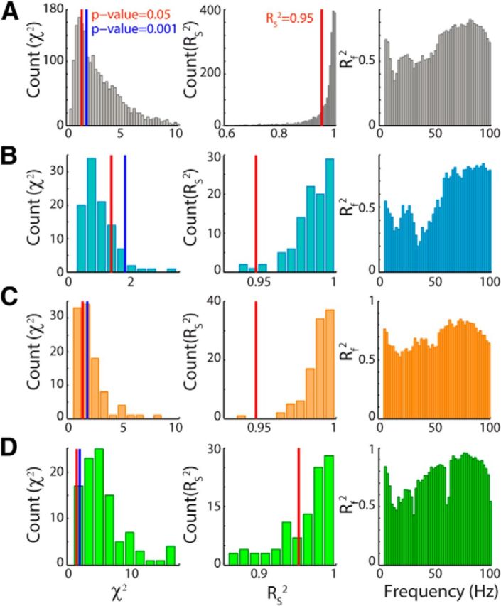
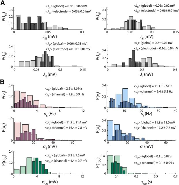
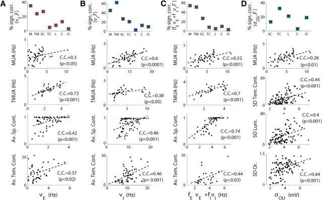
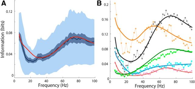
The local field potential (LFP) captures different neural processes, including integrative synaptic dynamics that cannot be observed by measuring only the spiking activity of small populations. Therefore, investigating how LFP power is modulated by external stimuli can offer important insights into sensory neural representations. However, gaining such insight requires developing data-driven computational models that can identify and disambiguate the neural contributions to the LFP. Here, we investigated how networks of excitatory and inhibitory integrate-and-fire neurons responding to time-dependent inputs can be used to interpret sensory modulations of LFP spectra. We computed analytically from such models the LFP spectra and the information that they convey about input and used these analytical expressions to fit the model to LFPs recorded in V1 of anesthetized macaques (Macaca mulatta) during the presentation of color movies. Our expressions explain 60%-98% of the variance of the LFP spectrum shape and its dependency upon movie scenes and we achieved this with realistic values for the best-fit parameters. In particular, synaptic best-fit parameters were compatible with experimental measurements and the predictions of firing rates, based only on the fit of LFP data, correlated with the multiunit spike rate recorded from the same location. Moreover, the parameters characterizing the input to the network across different movie scenes correlated with cross-scene changes of several image features. Our findings suggest that analytical descriptions of spiking neuron networks may become a crucial tool for the interpretation of field recordings.

Keywords: data-driven models; gamma oscillations; neural coding; primary visual cortex; recurrent networks; slow oscillations.

Figure 1.

Dynamics of a network receiving a time-dependent external input. Top to bottom, External input, raster plot of 200 excitatory neurons, average instantaneous excitatory firing rate, raster plot of the activity of 100 inhibitory neurons, average instantaneous inhibitory firing rate, and LFPs of the network modeled as the sum of AMPA and GABA currents on excitatory neurons. The external input is an OU process with average μ_OU = 20 mV, SD σ_OU = 10 mV, and time constant τ_OU = 100 ms. The parameters used in the simulations are those listen in the section “Numerical Integration Methods.”

Figure 2.

LFP power spectra: simulations versus theory. A, LFP power spectra in simulations and theory when using different values of the amplitude of the fluctuations around the mean input σ_OU = 0,3, 7 mV. The time constant of the OU process is kept fixed at τ_OU = 100 ms. The values of the others parameters are reported in the section “Numerical Integration Methods.” As the amplitude of the fluctuations increases, the values of the LFP power in the low-frequency range increase. B, LFP power SD as a function of the frequency in simulation and theory. The black curve is the SD calculated from the theoretical LFP power using the Welch formula σ² = 11L²/9K in which L is the mean LFP power and K is the number of windows used to calculate the LFP power in the simulations (K = 15). The red curve is the SD of the LFP power obtained from 40 simulations generated with different seeds. The blue curve represents the SD of the simulated LFP power calculated with the Welch formula. C, Information about the stimulus carried by the LFP power in simulation and theory. The information displays two well separated peaks: one in the low-frequency region due to the modulation of L_L,ext (Equation 39) by the external input and one in the gamma-frequency region due to the modulation of the finite-size term, L_L,FS (Equation 38).

Figure 3.

Test of the algorithm on synthetic data with free synaptic efficacies. A, Reduced χ² values versus Euclidean distance from the real parameter set obtained running the fitting algorithm starting from 50 different initial conditions. The red points correspond to χ² values with p < 0.05 and the black points to p > 0.05. The parameter set is composed by 10 parameters (ν_E, ν_I, σ_E, σ_I, σ_OU, τ_OU, J_EE, J_EI, J_IE, J_II). B, Distribution of the parameters describing the synaptic efficacies obtained by keeping only the cases in which the χ² had p < 0.05 (red points in A). Vertical lines denote median of the distribution (red) and true values of the parameters (black). C, Distributions of the parameters that depend on the input variations obtained by keeping only the cases in which the χ² had p < 0.05. Vertical lines are as in B. In both B and C, the distributions are broad, but the median values approximate well the values used to generate the data.

Figure 4.

Test of the algorithm on synthetic data with fixed synaptic efficacies. A, Reduced χ² values versus Euclidean distance from the real parameter set obtained running the fitting algorithm starting from 50 different initial conditions. The red points correspond to χ² values with p < 0.05 and the balck points to p > 0.05. The parameter set is composed by six parameters (ν_E, ν_I, σ_E, σ_I, σ_OU, τ_OU), whereas the synaptic efficacies are fixed at the median values of Figure 3. B, Distributions of the parameters that depend on the input variation calculated for the cases with χ² with p < 0.05 (red points in A). Vertical lines denote median of the ditribution (red) and true values of the parameters (black). The medians approximate well the values used to generate the data.

Figure 5.

Fitting procedure. Shown is a depiction of the second and final step of the fitting procedure. For each of the 100 scenes of a recording, the six scene-dependent parameters (ν_E, ν_I, σ_E, σ_I, σ_OU, τ_OU) were determined using the algorithm described in the text. The values of the synaptic efficacies (J_EE, J_EI, J_IE, J_II) were the same for all scenes and equal to the median values found in the first step of the fitting procedure. Therefore, for each scene, we evaluated six parameters using ∼50 values of the LFP power spectrum at the different frequencies.

Figure 6.

Quality of the fit of the experimental LFP power spectrum. A, Examples of the fits (solid curves) of the experimental LFP power spectrum (symbols) of three scenes with different degrees of the goodness of the fit: blue, purple, and green display, respectively, fit for which χ² < χ²(p = 0.05), χ²(p = 0.001), and χ² > χ²(p = 0.001). For the three examples of fit, the value of R_s² is higher than 0.95. Insert, Distribution of χ² over all scenes; red and blue vertical lines correspond, respectively, to the χ² with p = 0.05 and p = 0.001. B, Histograms of the percentages of well fitted scenes over all channels and sessions using three different criterions: χ² < χ²(p = 0.05) (left), χ² < χ²(p = 0.001) (middle), and R_s² > 0.95 (right). The percentage average of well fitted scenes in the three conditions is, respectively, equal to 28%, 43%, and 98%.

Figure 7.

χ² distribution and fraction of variance explained by the model. A, Left, χ² distribution over all of the scenes of all recordings. Middle, R_s² distribution over all scenes and all recordings. Right, R_f² versus frequency, calculated for each frequency as the median across recordings of the R_f² values. R_s² and R_f² are cross- validated measures of goodness of fit and represent the correlation between the mean values over half of the trials of the observed LFP power and the corresponding values of the fit obtained using the other half of the data sample. B, Same quantities as in A, but for a single recording in which the majority of scenes has χ² < χ²(p = 0.001). C, Same quantities as in A, but for a single recording in which only a fraction of scenes has χ² < χ²(p = 0.001). D, Same quantities as in A, but for a single recording in which the majority of scenes has χ² > χ²(p = 0.001).

Figure 8.

Distributions of the parameters found through the fitting procedure. A, Each panel shows the distribution of a single synaptic efficacy found through the fitting procedure over all the recordings (light gray) and over the channels of a single electrode (dark gray). B, Distribution of the parameters that can vary from scene to scene over all the scenes of all the recordings (light bars) and over all the scenes of a single recording (dark bars).

Figure 9.

Correlations between the parameters extracted from fit and the experimental observables. A, Top, Percentages of recordings with significant correlation under the condition χ² < χ²(p = 0.001) between the excitatory firing rate found through the fits and the experimental observables on the x-axis: MUA of a single channel (M); MUA of all the channels of a single experimental session (TM); average spatial contrast (SC), average temporal contrast (TC), luminance (L), orientation (O), and color (C). On the other four panels are displayed some examples in which these correlations were found. B, Same as in A, but for correlations with inhibitory firing rates extracted from fits. C Same as in A, but for correlations with total firing rate. D, Same as in A, but for the correlations between the amplitude of the fluctuations of the OU process, σ_OU, that was found through the fits and the SDs of the different features of the movie.

Figure 10.

Information content of the LFP power. A, Information content of the experimental LFP power (blue solid line represents the mean, whereas the light (dark)-shaded area represents mean ± std (SE) across 37 different recordings compared with the mean across all recordings of the theoretical information (red solid line), which was calculated using Equation 13 with the LFP power values found through the fitting procedure. B, Some examples of information carried by the LFP power of a single recording channel in experiment (symbols) and theory (solid curves).

References

1. Abramowitz M, Stegun IA. Tables of mathematical functions. New York: Dover Publications; 1970.
1. Anderson JS, Lampl I, Gillespie DC, Ferster D. The contribution of noise to contrast invariance of orientation tuning in cat visual cortex. Science. 2000;290:1968–1972. doi: 10.1126/science.290.5498.1968. - DOI - PubMed
1. Bair W, Koch C, Newsome W, Britten K. Power spectrum analysis of bursting cells in area MT in the behaving monkey. J Neurosci. 1994;14:2870–2892. - PMC - PubMed
1. Bartels A, Zeki S, Logothetis NK. Natural vision reveals regional specialization to local motion and to contrast-invariant, global flow in the human brain. Cereb Cortex. 2008;18:705–717. doi: 10.1093/cercor/bhm107. - DOI - PubMed
1. Bartos M, Vida I, Frotscher M, Geiger JR, Jonas P. Rapid signaling at inhibitory synapses in a dendate gyrus interneuron network. J Neurosci. 2001;21:2687–2698. - PMC - PubMed
Publication types
LinkOut - more resources