

doi: 10.1109/MSP.2010.936730.
Machine Learning in Medical Imaging
- PMID: 25382956
- PMCID: PMC4220564
- DOI: 10.1109/MSP.2010.936730
Item in Clipboard
Machine Learning in Medical Imaging
IEEE Signal Process Mag.
2010 Jul.
No abstract available
Figures
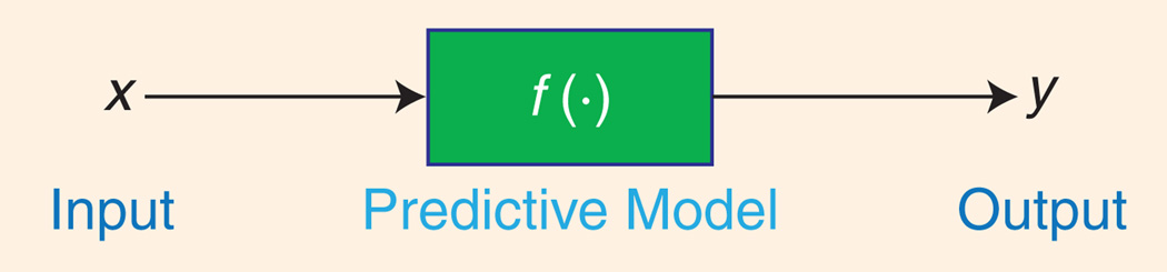
In supervised learning the predictive model represents the assumed relationship between input variables in x and output variabley.

Fisher linear discriminant (LD) and the SVM. In this example, (a) the Fisher LD fails to separate two classes because training example D adversely influences decision boundary T. (b) The SVM defines the decision boundary using only points A, B, and C, called support vectors, and is not influenced at all by point D.

(a) Example mammogram containing microcalcifications. (b) Output y of SVM detector. (c) Detected MC positions obtained by thresholding y.

(a) Comparison of support vectors from SVM and (b) relevance vectors from RVM for detection of MCs. SVM automatically chooses the support vectors to be examples lying near the decision boundary (hence the “MC absent” and “MC present” support vectors look very similar), while the relevance vectors chosen by RVM tend to be more prototypical of the two classes (hence the two groups of relevance vectors look very different).

Detection performance of various methods of detecting MCs in mammograms. The best performance was obtained by a successive learning SVM classifier, which achieves around 94% detection rate (TP fraction) at a cost of one FP cluster per image, where a classical technique (DoG) achieves a detection rate of only about 68%.

Statistical tool for visualizing relationships among abnormalities seen in various mammograms, in which distances reflect the relative similarities of abnormalities, as judged by human experts. MC clusters are represented in this two-dimensional diagram by using multidimensional scaling, a statistical technique that seeks to represent high-dimensional data in a lower-dimensional plot that can be readily visualized, while aiming to maintain the relative distances (similarities) among the data points. Each group of red plus signs (+) depicts the actual MC cluster associated with a given point in the scatter plot. This shows that the vertical axis of the plot is roughly associated with the density of each cluster, while the horizontal axis is related to its shape.
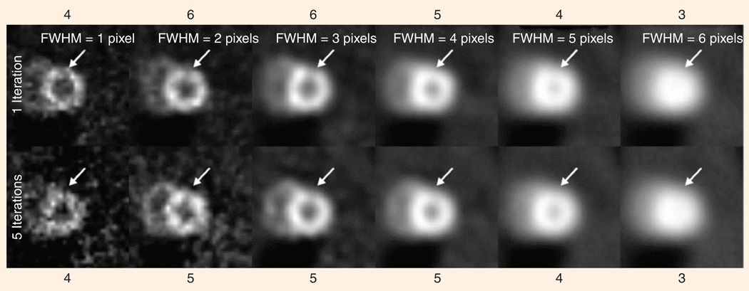
A human observer’s judgment as to the presence of an abnormality (in this case a cardiac perfusion defect) depends on the parameters of the reconstruction algorithm used to create the image (here, the parameters are number of iterations and width (FWHM) of the post-reconstruction smoothing kernel). All of the images above have a defect at the location indicated by the arrow, but persons asked to judge whether there is a defect varied in their opinions from a value of three, meaning “defect is possibly not present,” to a value of six, meaning “defect is definitely present.” Our algorithm’s ability to predict this behavior permits us to optimize a given algorithm for this specific diagnostic task.
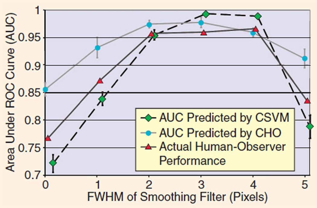
Predictions of human-observer performance (AUC) by machine learning approach (CSVM) compared with conventional numerical observer (CHO). The CHO does not recognize the degree to which diagnostic performance declines at low and high levels of smoothing, an effect seen in scores along the top and bottom of Figure 7
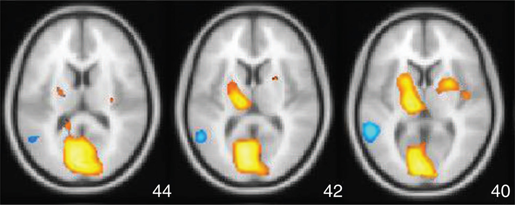
Spatial activation pattern in the brain, showing effect of the anxiolytic/antidespressant drug buspirone (Buspar) obtained using Fisher LD and NPAIRS split-half resampling applied to FDG-PET images for 12 subjects (data courtesy of Abiant, Inc.; analysis by Predictek, Inc.). The results show striatal activation (upper orange regions), likely due to the drug’s behavior as a dopamine D2 receptor antagonist.
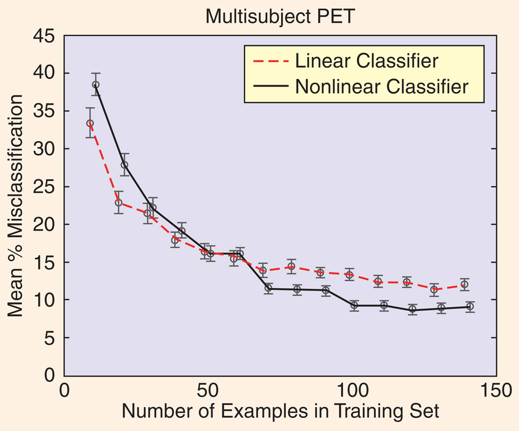
These crossed learning curves (plots of classifier performance versus training set size) show that a nonlinear classifier (a neural network in this example) can be beaten by a simpler multivariate linear classifier (here, a Fisher discriminant) when the number of training examples is small. This is not unexpected, as small data sets cannot generally support complex models, however this result emphasizes the importance of resisting the temptation for researchers to use high-complexity models in every circumstance.

Simulated phantom used for testing signal detection.

In (a)–(c), performance in detection of brain activation for five models, as a function of signal-to-noise variance ratio (V) and correlations (rho) among network of activated brain regions, are shown. The QD and NLD perform best, improving with strength of network (increasing V and rho), while the performance of univariate methods lags behind, and actually deteriorates as the signal strength increases.
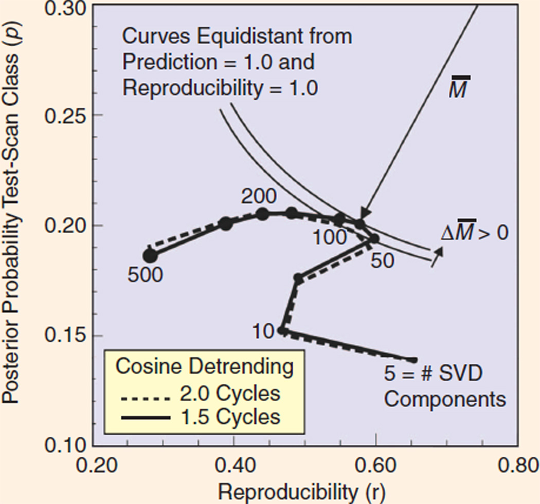
In the NPAIRS framework, a prediction-reproducibility (p,r) curve shows the tradeoff between prediction accuracy (vertical axis) and reproducibility of the resulting brain map (horizontal axis). Optimal performance is achieved when the curve comes closest to the ideal point (1,1), achieving the smallest distance M̅. This provides a basis for optimizing image analysis procedures, in this example specifying the best parameters in a particular fMRI data analysis problem (number of SVD components and number of cycles in a particular cosine detrending step).
References
-
- Hastie T, Tibshirani R, Friedman JH. The Elements of Statistical Learning. New York: Springer-Verlag; 2003.
-
- Scholkopf B, Smola AJ. Learning with Kernels: Support Vector Machines, Regularization, Optimization, and Beyond. Cambridge, MA: MIT Press; 2001. p. 626.
-
- Wernick MN. “Pattern classification by convex analysis”. J. Opt. Soc. Amer. A, Opt. Image Sci. 1991;8:1874–1880.
-
- Vapnik VN. Statistical Learning Theory. New York: Wiley; 1998.
-
- Tipping ME. “Sparse Bayesian learning and the relevance vector machine”. J. Mach. Learn. Res. 2001 Sep;1:211–244.
Grants and funding
LinkOut - more resources
Full Text Sources
Other Literature Sources