Functional transformations of odor inputs in the mouse olfactory bulb

Abstract

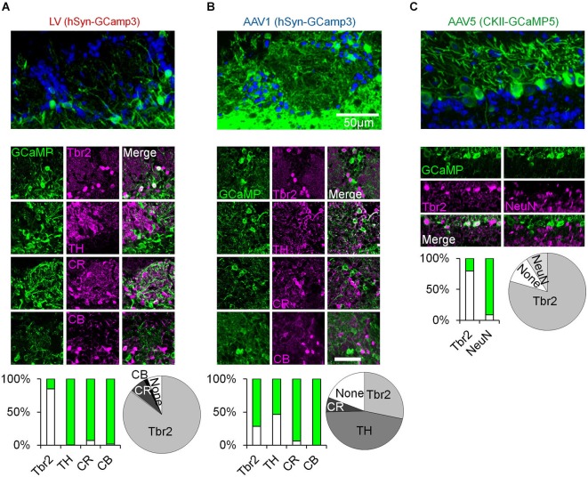
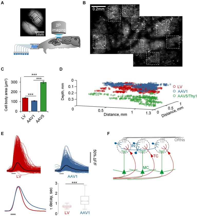
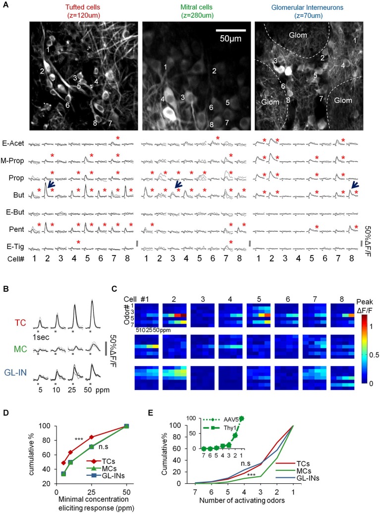
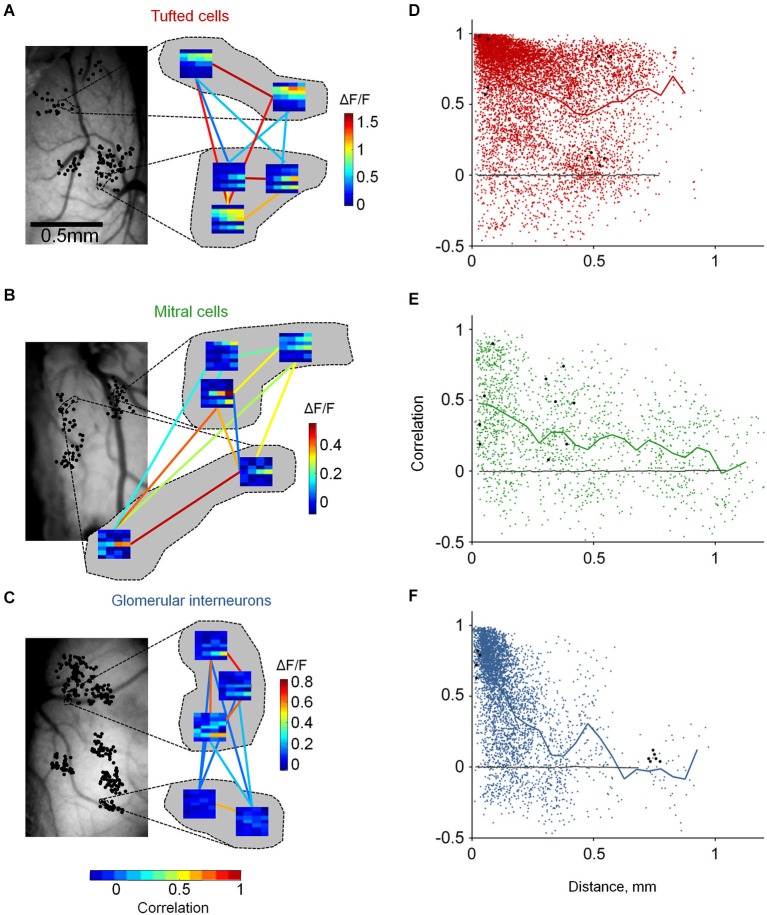
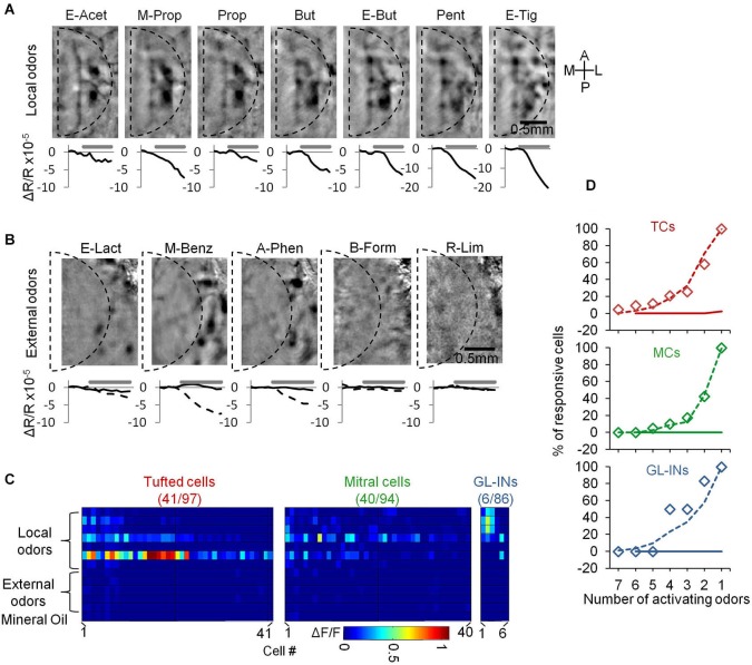
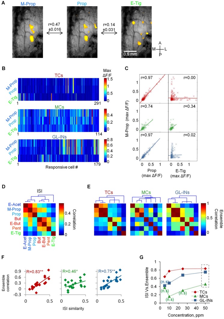
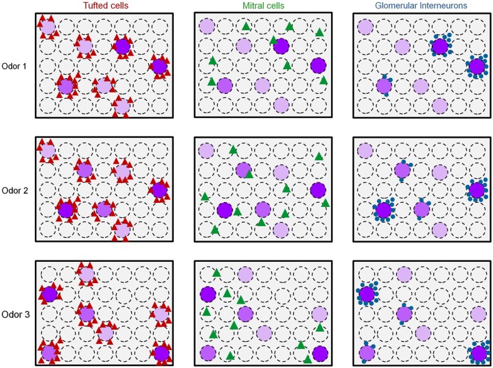
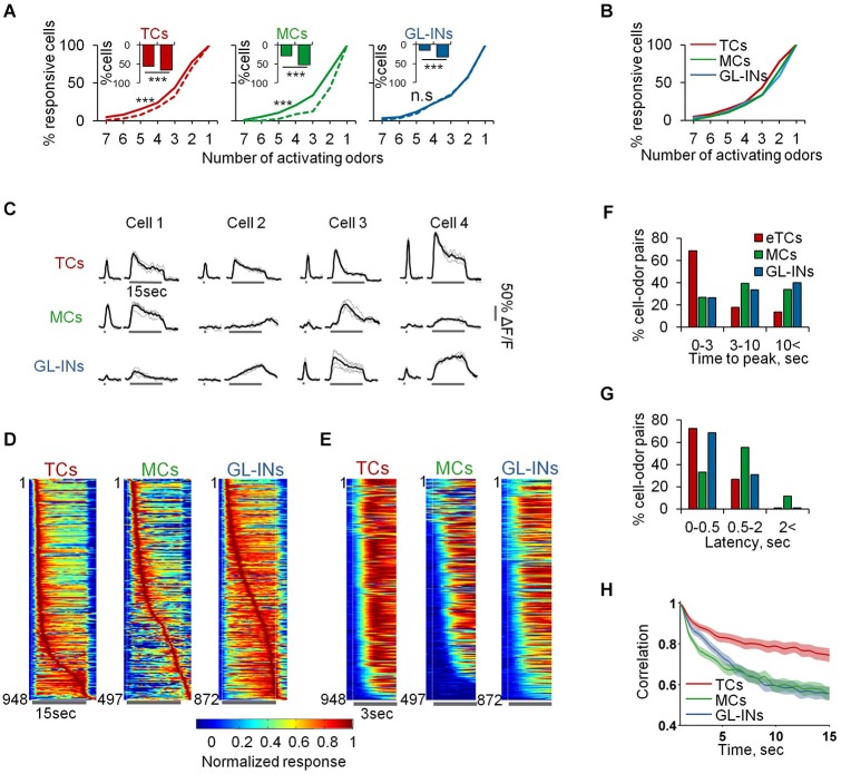
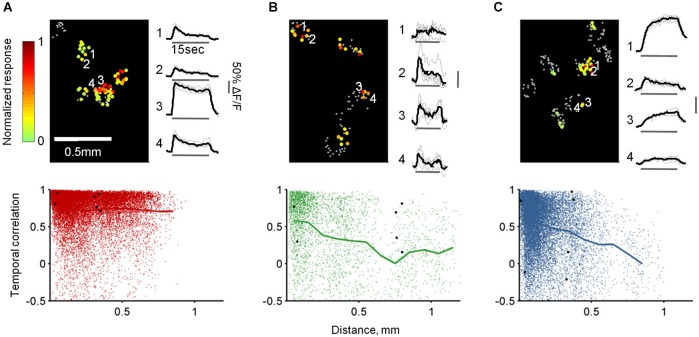
Sensory inputs from the nasal epithelium to the olfactory bulb (OB) are organized as a discrete map in the glomerular layer (GL). This map is then modulated by distinct types of local neurons and transmitted to higher brain areas via mitral and tufted cells. Little is known about the functional organization of the circuits downstream of glomeruli. We used in vivo two-photon calcium imaging for large scale functional mapping of distinct neuronal populations in the mouse OB, at single cell resolution. Specifically, we imaged odor responses of mitral cells (MCs), tufted cells (TCs) and glomerular interneurons (GL-INs). Mitral cells population activity was heterogeneous and only mildly correlated with the olfactory receptor neuron (ORN) inputs, supporting the view that discrete input maps undergo significant transformations at the output level of the OB. In contrast, population activity profiles of TCs were dense, and highly correlated with the odor inputs in both space and time. Glomerular interneurons were also highly correlated with the ORN inputs, but showed higher activation thresholds suggesting that these neurons are driven by strongly activated glomeruli. Temporally, upon persistent odor exposure, TCs quickly adapted. In contrast, both MCs and GL-INs showed diverse temporal response patterns, suggesting that GL-INs could contribute to the transformations MCs undergo at slow time scales. Our data suggest that sensory odor maps are transformed by TCs and MCs in different ways forming two distinct and parallel information streams.

Keywords: calcium imaging; functional organization; in vivo imaging; neuronal populations; olfactory bulb.

Figure 1

Immunohistochemical analysis of OB cell types labeled with distinct viral vectors. (A–C) Top, confocal micrographs from the OB following virus injection. Middle, representative images of GCaMP expression and its overlap with Tbr2 (Winpenny et al., 2011), TH, Calretinin (CR), and Calbindin (CB) positive neurons (Parrish-Aungst et al., ; Adam and Mizrahi, 2011). Green images—expression of GCaMP. Magenta images—Staining with antibodies against the indicated marker. Merged images—double labeling of GCaMP and the respective marker. Bar graphs—percent of double labeling between GCaMP and the indicated marker (Green = GCaMP positive and marker negative, white = GCaMP positive and marker positive). Pie charts—summary of the composition of each sample (based on the bar graphs). LV—Lentivirus, AAV—adeno-associated virus, hSyn—human synapsin promoter, CKII—CamKII promoter. Tbr2—T-Brain gene 2, TH—tyrosine hydroxylase, CR—calretinin, CB—calbindin, NeuN—neuronal nuclear marker.

Figure 2

Functional mapping of TCs, GL-INs and MCs. (A) Experimental setup. Schematic of an anesthetized mouse implanted with a chronic imaging window placed under the two-photon microscope. Mice were stimulated with seven odorants, delivered through an olfactometer with completely separate channels. The image is a still image of both bulbs in a representative chronic window. (B) Two consecutive low resolution two-photon micrographs of cells expressing GCaMP3 after infection with AAV1-hSyn-GCaMP3. Images are from the same OB shown in (A) (where imaged regions on the blood vessel map are denoted by black dotted squares). In this OB, eight imaging fields were used for imaging (white dotted squares). (C) Quantification of the 2D area of cell bodies labeled and imaged with the different viruses (mean ± S.E.M, n = 91 TCs, n = 79 GL-INs, n = 55 MCs, ***p < 0.001, T-test). (D) Depth from the surface of all cells imaged in this study (TCs—130 ± 26 µm, GL-INs—82 ± 21 µm, MCs—270 ± 41 µm). Locations of cells are aligned within mice. (E) Top, Calcium transients of all cell-odor pairs from LV and AAV1 infected neurons (black line = mean). Bottom left, normalized mean transients. Bottom right, Distribution of the mean τ decay of all cells. Tufted cells decays were faster and homogenous. In agreement with the heterogeneous nature of the GL-INs, their τ decays were highly heterogeneous and significantly slower compared with TCs (n = 298 TCs and n = 189 GL-INs). Box shows the 25 to 75 percentile, line = median, bars show the data limits. *** p < 0.001, unpaired T-test. (F) Scheme of the OB circuit and the cell types studied in this work.

Figure 3

Basic response properties of TCs, GL-INs and MCs. (A) Two-photon micrographs of fields used for calcium imaging, and a sample of calcium transients elicited in eight representative neurons in the field (cells marked by numbers) by the different odorants (at 50 ppm). Gray traces—single trials, Black traces—mean response. Stimulus duration = 1 s. Red asterisk = statistically significant response (see Section Methods). (B) Examples of responses to four concentrations of butanal in single cell odor pairs from each population (cell-odor pairs are denoted by arrows in (A)). Gray traces—single trials, Black trace—average. (C) Full response profiles of the same cells shown in (A) (for a total of 24 neurons). Rows = odors, columns = concentrations. Colorcode = max ΔF/F. (D) Response thresholds, cumulative graphs of the lowest concentration eliciting response in each cell. Tufted cells are activated at significantly lower concentration (***p < 0.001, T-test). (E) Odor selectivity. Cumulative graphs of the number of activating odors (only for cells responding to at least one odor). Mitral cells response profiles are sparser compared to TCs and GL-INs (***p < 0.001 T-test). Inset, selectivity of MCs labeled with AAV5-GCaMP5 (dotted line) vs. Thy1-GCaMP3 (dashed line).

Figure 4

Distinct functional architecture of TCs, GL-INs and MCs. (A)—TCs, (B)—MCs, (C)—GL-INs. Left, still image of the blood vessels on the dorsal surface of the OB. Black dots denote the location of all imaged cells (in a 2D dorsal view). Dashed lines mark the location of the cells which their enlarged response profiles are shown on the right. Right, examples of response profiles from five neurons in each OB. Each row represent one odor (1-E-Acet, 2-M-Prop, 3-Prop, 4-But, 5-E-But, 6-Pent, 7-E-Tig), and each column represents a single concentration (5, 10, 25, 50 ppm). Color-code (vertical) is the max ΔF/F in each condition. Colored lines represent the signal correlation between the connected cells, represented by the horizontal color bar. (D)—TCs, (E)—MCs, (F)—GL-INs. Signal correlation between the response profiles of all pairs as a function of the distance between the cells. Thick line—mean correlation averaged in 50 µm bins. Black dots—the example pairs from (A) (B) or (C). Black line—correlation between randomly shuffled response profiles. TCs: n = 8755 pairs from n = 306 active neurons in six OBs, GL-INs: n = 4128 pairs from n = 194 active neurons in six OBs, MCs: n = 1682 pairs from n = 149 active neurons in 10 OBs.

Figure 5

Neurons from the dorsal surface are not activated by distant glomeruli. (A) Intrinsic signal imaging maps showing activation by the panel of odorants used in this study. The borders of a standard chronic imaging window are denoted by the dashed line. Beneath each map we show the dynamics of the intrinsic signal before and during a 4 s stimulus. Signal is the sum intrinsic signal within the dashed line. (B) Same as in (A) but for five “external” odors. Curves in the bottom shows the dynamics of the intrinsic signal within the window (black) and outside the window (dashed). (C) Calcium responses of all responsive neurons that were tested with both “local” and “external” odor sets. Color-code—Peak ΔF/F. Cells in each population are sorted according to the number of activating odorants. Only the responsive cells in each group are presented (total numbers are outlined in the title of each panel). (D) Cumulative graphs of the number of activating odors in each population (responsive cells only). Diamonds—local odors from this dataset, dashed line—local odors in the main dataset (same as Figure 3E), solid line—external odors.

Figure 6

Input-output relationships of TCs, GL-INs and MC ensembles. (A) Representative intrinsic signal imaging maps in response to three different odors from one OB. Maps were filtered to represent ORNs input (see Section Methods). r = Pearson correlation between the intrinsic signal maps across the data (mean ± S.E.M, n = 36 OBs; n = 252 maps). (B) Ensemble calcium activity for three odors in the three neuronal populations. Only responsive cells are shown (TCs, n = 291 cells, GL-INs, n = 179 cells, MCs, n = 114 cells). (C) Max ΔF/F for M-Prop as a function of max ΔF/F for Prop (left column) or E-tig (right column). r = correlation between the ensemble responses to the odor pairs. (D) Correlation of all odor pairs at the ORN level, calculated as in (A) from the intrinsic signal maps. Dendrogram shows hierarchal clustering of the correlation values. The three clusters are represented by color in the odor names (blue, red, and green). ISI—Intrinsic signal imaging. (E) Ensemble correlation for all odor pairs in the three neuronal populations. Dendrograms show hierarchical clustering of the correlation values. Odors as in (D). The intrinsic signal clusters are preserved in the TCs but not in the MCs. (F) Ensemble correlation of each population at 50 ppm concentration (as in C and E) were plotted as a function of the correlations between the ORNs input (as in A and D). r = Pearson correlations between both vectors. **p < 0.01, *p < 0.05. ISI—Intrinsic signal imaging. (G) Correlation between the intrinsic signal similarity and the ensemble correlation (as presented in panel F) as a function of the odor concentration (n.s–non-significant correlation values).

Figure 7

Early spatiotemporal transformations in the olfactory bulb. Scheme of the putative functional organization of the different cell types in the OB to distinct odors. Dashed circles represent glomeruli. Purple glomeruli are responsive to an odor, and the purple color intensity represents the strength of glomerular activation. Odor 1 and odor 2 induce similar glomerular activation patterns while odor 3 activates a different set of glomeruli. Red triangles = Responsive TCs, Green triangles = Responsive MCs, Blue circles = responsive GL-INs.

Figure 8

Slow temporal dynamics of TCs, GL-INs and MCs. (A) Odor selectivity graphs for 1 s (dashed) vs. 15 s (solid) stimuli (***p < 0.001, Kolmogorov-Smirnov test). Inset shows the responsiveness at 1 (left bar) vs. 15 (rightbar) second odor stimulus. All populations are more responsive for the longer stimulus (***p < 0.001, Chi² test). (B) Odor selectivity graph for 15 s stimuli only. Same as solid line in (A). (C) Examples for traces of cell odor pairs at 1 and 15 s odor stimuli. All traces show the responses of different cells from a single OB to the same odor (Butanal). Gray—single trials, Black—mean response. (D) Time course for all the responsive cell-odor pairs, normalized to the peak and sorted by the time to peak. (E) Time course for all the responsive cell-odor pairs, normalized and sorted by the response latency. (F) Distribution of the time to peak, corresponding to the data in (D). (G) Distribution of the response latency, corresponding to the data in (E). (H) Correlation of the cell ensembles with the initial response pattern over time, averaged across all odors and OBs (mean ± SEM).

Figure 9

Spatiotemporal response patterns of TCs, GL-INs and MCs. (A)—TCs, (B)—MCs and (C)—GL-INs. Top left—activation map from a single OB for a single odor (Butanal). Each cell is denoted by a dot, gray dots represent non-responsive cells, color-code represent the peak ΔF/F for 15 s stimulation with Butanal. Responses in each bulb were normalized to the highest response. Top right—example of the response traces for four cells (marked by a number on the map). Gray—single trials; black—mean response. Bottom—correlation of the response patterns of all pairs of cells responding to the same odor in each bulb (up to seven odors for a pair), plotted as a function of the distance between the cells (TCs, n = 19918 pairs from six OBs, GL-INs—16383 pairs from six OBs, MCs—3229 pairs from 10 OBs). Thick line—mean correlation binned every 100 µm. Black dots—correlation between all possible pairs of the cells from the examples in the top panels.

References

1. Abraham N. M., Spors H., Carleton A., Margrie T. W., Kuner T., Schaefer A. T. (2004). Maintaining accuracy at the expense of speed: stimulus similarity defines odor discrimination time in mice. Neuron 44, 865–876. 10.1016/j.neuron.2004.11.017 - DOI - PubMed
1. Adam Y., Mizrahi A. (2010). Circuit formation and maintenance–perspectives from the mammalian olfactory bulb. Curr. Opin. Neurobiol. 20, 134–140. 10.1016/j.conb.2009.11.001 - DOI - PubMed
1. Adam Y., Mizrahi A. (2011). Long-term imaging reveals dynamic changes in the neuronal composition of the glomerular layer. J. Neurosci. 31, 7967–7973. 10.1523/jneurosci.0782-11.2011 - DOI - PMC - PubMed
1. Akerboom J., Chen T. W., Wardill T. J., Tian L., Marvin J. S., Mutlu S., et al. . (2012). Optimization of a GCaMP calcium indicator for neural activity imaging. J. Neurosci. 32, 13819–13840. 10.1523/JNEUROSCI.2601-12.2012 - DOI - PMC - PubMed
1. Aungst J. L., Heyward P. M., Puche A. C., Karnup S. V., Hayar A., Szabo G., et al. . (2003). Centre-surround inhibition among olfactory bulb glomeruli. Nature 426, 623–629. 10.1038/nature02185 - DOI - PubMed
Publication types
LinkOut - more resources