Evolutionary tipping points in the capacity to adapt to environmental change

Abstract

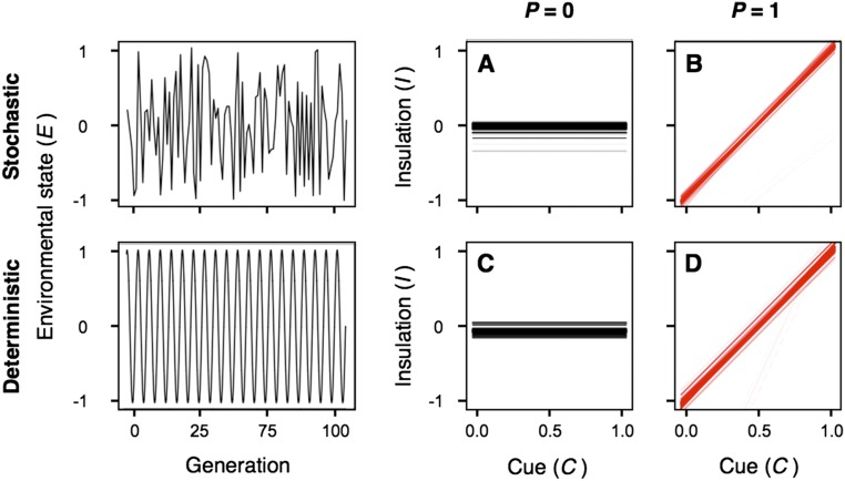
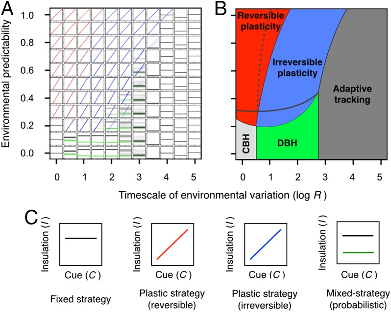
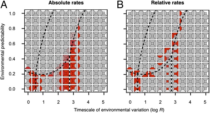
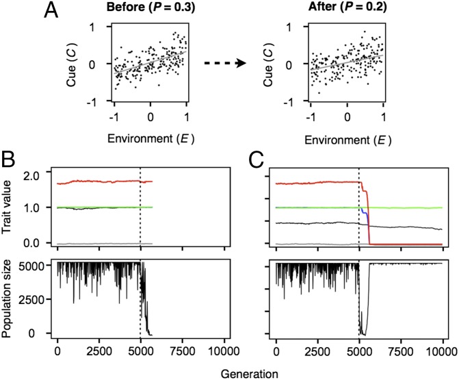
In an era of rapid climate change, there is a pressing need to understand how organisms will cope with faster and less predictable variation in environmental conditions. Here we develop a unifying model that predicts evolutionary responses to environmentally driven fluctuating selection and use this theoretical framework to explore the potential consequences of altered environmental cycles. We first show that the parameter space determined by different combinations of predictability and timescale of environmental variation is partitioned into distinct regions where a single mode of response (reversible phenotypic plasticity, irreversible phenotypic plasticity, bet-hedging, or adaptive tracking) has a clear selective advantage over all others. We then demonstrate that, although significant environmental changes within these regions can be accommodated by evolution, most changes that involve transitions between regions result in rapid population collapse and often extinction. Thus, the boundaries between response mode regions in our model correspond to evolutionary tipping points, where even minor changes in environmental parameters can have dramatic and disproportionate consequences on population viability. Finally, we discuss how different life histories and genetic architectures may influence the location of tipping points in parameter space and the likelihood of extinction during such transitions. These insights can help identify and address some of the cryptic threats to natural populations that are likely to result from any natural or human-induced change in environmental conditions. They also demonstrate the potential value of evolutionary thinking in the study of global climate change.

Keywords: adaptive tracking; bet-hedging; fluctuating selection; global change; phenotypic plasticity.

Fig. 1.

Effects of environmental stochasticity on the evolution of thermal strategies when environments are either completely unpredictable (A and C) or completely predictable (B and D). Stochastic environmental variation (A and B) was modeled by setting the value of weighting constants to A = 0 and B = 1. Conversely, comparable deterministic variation (C and D) was modeled through A = 1, B = 0, and R = 1. The norm of reaction plots depict the strategies of 5,000 individuals at generation 50,000 in representative replicate simulation runs. Darker colors indicate that a higher number of individuals share a given response to a particular environmental cue. Comparison of the top and bottom panels indicates that the way in which environments vary, stochastically vs. deterministically, is less important to evolution than the degree to which individuals can anticipate such variation.

Fig. 2.

Evolutionary response to environmental variation under different levels of predictability (P) and relative timescale of environmental variation (R). At each parameter combination in A, the 100 mean population reaction norms that evolved at generation 50,000 in different replicate simulations are depicted as in Fig. 1 with environmental cues on the x axis and the resulting insulation phenotypes on the y axis (labels omitted for simplicity). If only one reaction norm is visible, this is an indication that the same response evolved in all replicates. As illustrated in C, reaction norms are depicted in black when $\overline{s}\le 0.5$ (see Table S1 for details). In such a case, phenotypic plasticity does not occur (a is not expressed) and the reaction norm is flat. In case of a plastic response ($\overline{s}>0.5$), reaction norms are depicted in a color gradient ranging from red when $\overline{a}=1$ (reversible plasticity) to blue when $\overline{a}=0$ (irreversible plasticity). For simplicity, secondary reaction norms are depicted in green with intensity proportional to how often they are used (i.e., they are not visible if $\overline{h}=1$). (B) The consistency of outcomes across replicates in A suggests that different regions in parameter space favor different modes of response. Conservative and diversifying bet-hedging are identified in B as CBH and DBH, respectively. Dashed gray lines in B depict changes in the boundaries between different adaptive regions when adjustment costs, k_a, are doubled from 0.01 to 0.02, and solid gray lines depict changes when the cost of development, k_d, is doubled from 0.02 to 0.04.

Fig. 3.

Rates of extinction when transitioning into nearby regions of parameter space when q = 2.2. Each subplot within each panel depicts the baseline level of extinction at a given parameter combination (inner square), and the extinction rates associated with transitioning into the nearest parameter combination to the top, bottom, left, and right of that cell (trapezoids). The boundaries between response mode regions in Fig. 2B are presented as dashed lines. (A) We use a color gradient from gray (0%) to red (100%) to depict absolute extinction rates (i.e., the proportion of simulations that went extinct during 100 replicate transition runs). (B) Relative rates were computed as (TR − BR)/BR, where TR = transition rate of extinction, and BR = baseline rate of extinction at the target parameter combination (i.e., where the population is moving into). The color scale for these rates ranges from blue (≤−100%) to red (≥100%). The absence of blue trapezoids in B indicates that, in practice, transition rates were always similar or greater than their corresponding baselines.

Fig. 4.

Representative examples of population dynamics during transitions through evolutionary tipping points in our model. (A) In the simulations depicted here, populations were forced to move from the region of reversible plasticity into that of bet-hedging by lowering P from 0.3 to 0.2 at log R = 0 (all other model parameters as in the main text). (Top) Change in the correlation between cues and environmental values. (Middle) Evolution of traits before and after the transition (black = s, blue = a, green = h, gray = I₀, and red = b; the time of transition is depicted by a dashed vertical line at generation 5,000). (Bottom) Associated changes in population size over time. (A) Even though the change in predictability is barely visible to the naked eye, populations immediately decline after predictability is reduced. (B) In most situations, populations become extinct because the mutations required to adapt to the new environment fail to arise. (C) However, in cases where beneficial mutations arise on time, these traits tend to reach fixation quickly and evolutionary rescue is complete.

References

1. Parmesan C. Ecological and evolutionary responses to recent climate change. Annu Rev Ecol Evol Syst. 2006;37:637–669.
1. Piersma T, van Gils JA. The Flexible Phenotype: A Body-Centred Integration of Ecology, Physiology, and Behaviour. Oxford Univ Press; New York: 2010. p 248.
1. Moritz C, Agudo R. The future of species under climate change: Resilience or decline? Science. 2013;341(6145):504–508. - PubMed
1. Hoffmann AA, Sgrò CM. Climate change and evolutionary adaptation. Nature. 2011;470(7335):479–485. - PubMed
1. Bradshaw WE, Holzapfel CM. Climate change. Evolutionary response to rapid climate change. Science. 2006;312(5779):1477–1478. - PubMed
Publication types
LinkOut - more resources