

doi: 10.1177/108471389600100102.
Theoretical and practical considerations in compression hearing AIDS
Affiliations
- PMID: 25425854
- PMCID: PMC4172289
- DOI: 10.1177/108471389600100102
Item in Clipboard
Theoretical and practical considerations in compression hearing AIDS
Trends Amplif.
1996 Mar.
No abstract available
Figures
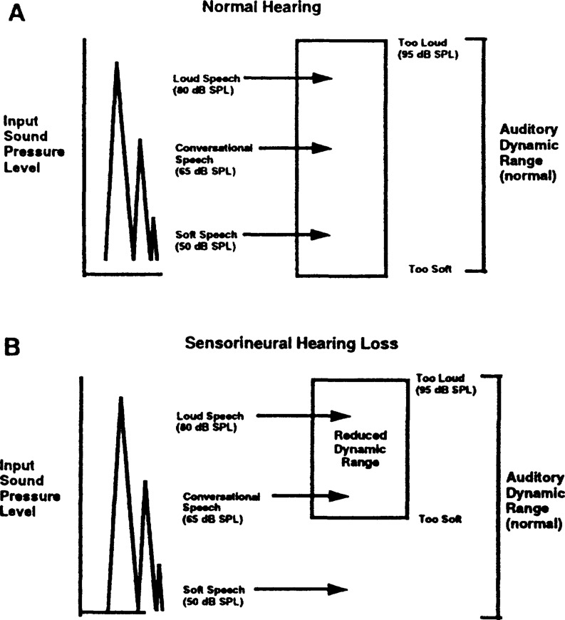
Representation of soft, conversational and loud speech into the auditory dynamic range (A) normal hearing, (B) sensorineural hearing loss.
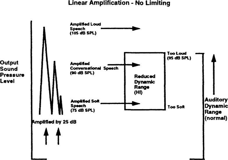
Example to show how linear amplification without limiting (25 dB gain), when applied to soft, conversational and loud speech, may alter its representation in the residual auditory dynamic range of a hearing-impaired ear.
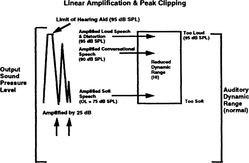
Example to show how linear amplification with peak clipping (25 dB gain), when applied to soft, conversational, and loud speech, may affect its representation in the residual auditory dynamic range of a hearing-impaired ear.
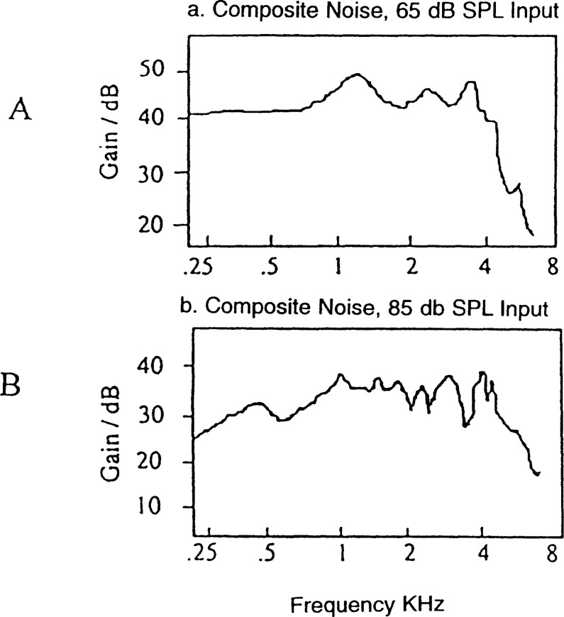
Frequency response curves of a hearing aid with linear amplification when tested with composite noise at (A) 65 dB SPL, and (B) 85 dB SPL (hearing aid in saturation).
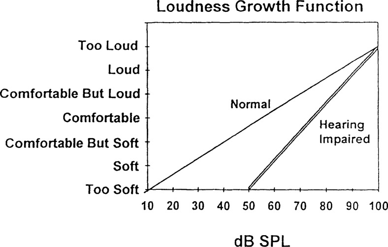
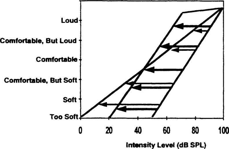
Hypothetical loudness growth functions for a normal hearing listener and hearing-impaired listener.
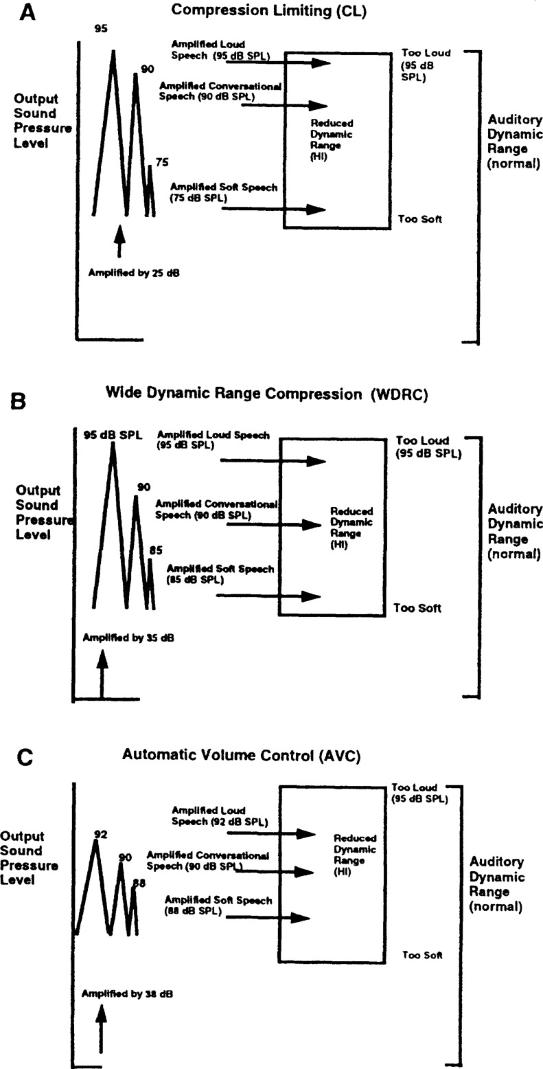
Three approaches to “compress” the entire speech range into the residual auditory dynamic range of the hearing-impaired ear: (A) compression limiting (CL), (B) wide dynamic range compression (WDRC), and (C) automatic volume control (AVC).
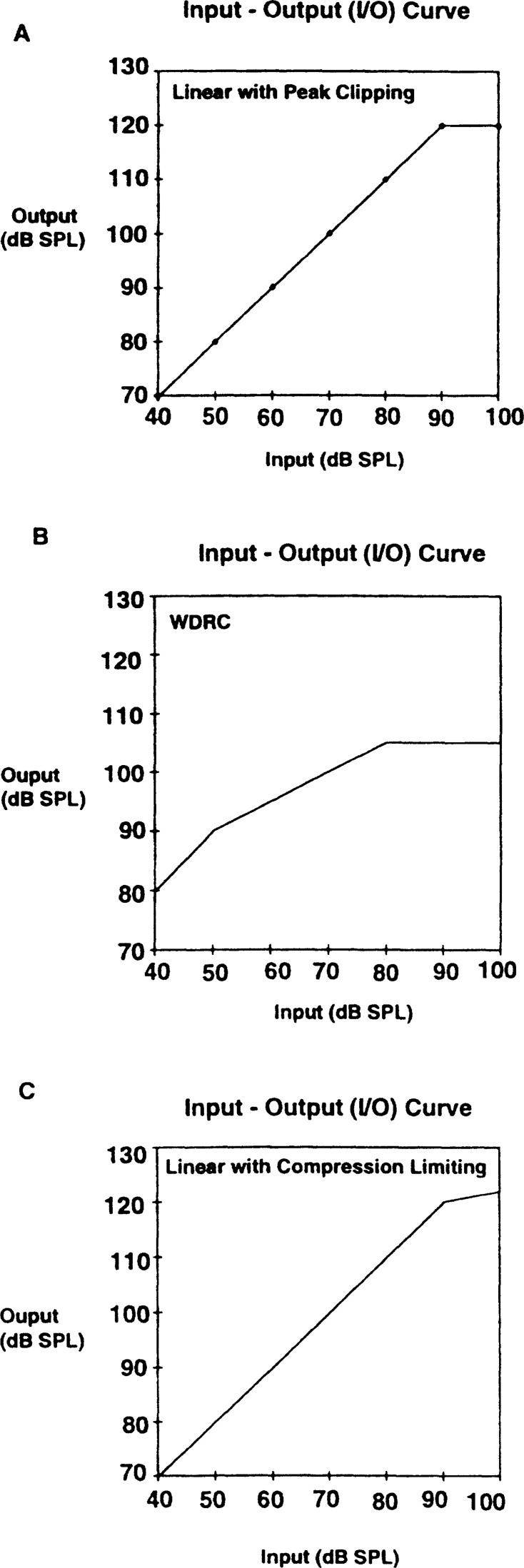
Input-output (I-O) curves of different hearing aids. (A) Linear with peak clipping, (B) wide dynamic range compression, and (C) compression limiting.
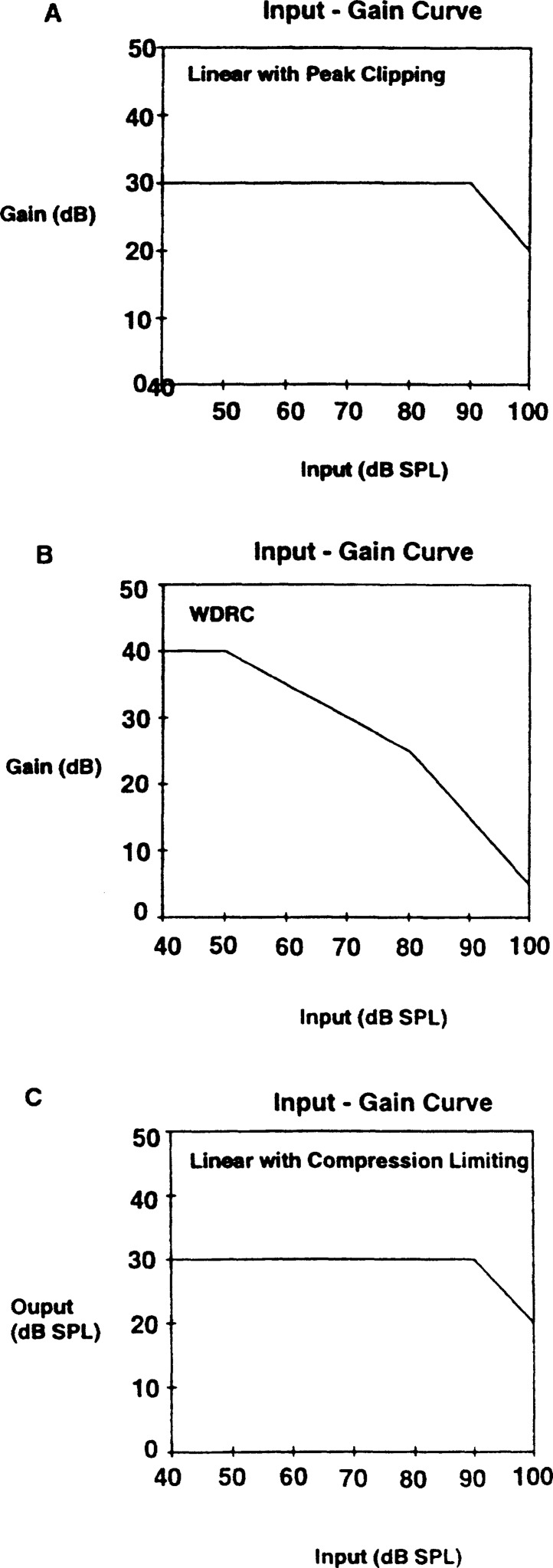
Input-gain curves of the hearing aids shown in Figure 7: (A) Linear with peak clipping, (B) wide dynamic range compression, and (C) compression limiting.
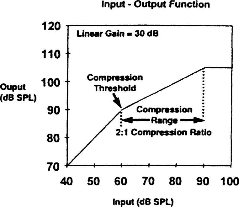
Input-output curve showing the different static compression characteristics.
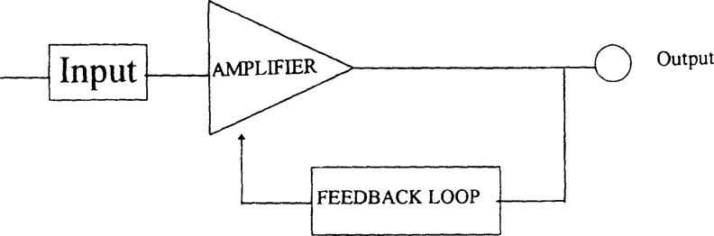
Schematic diagram of a compression circuit.
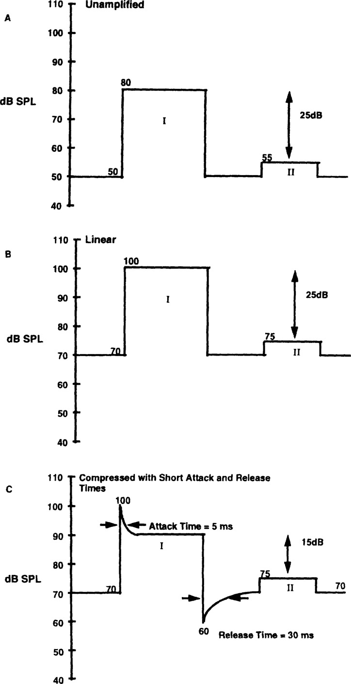
Illustration of attack and release times and associated output waveform from a compression hearing aid: (A) unamplified signal (B) linearly amplified output, and (C) compressed output.
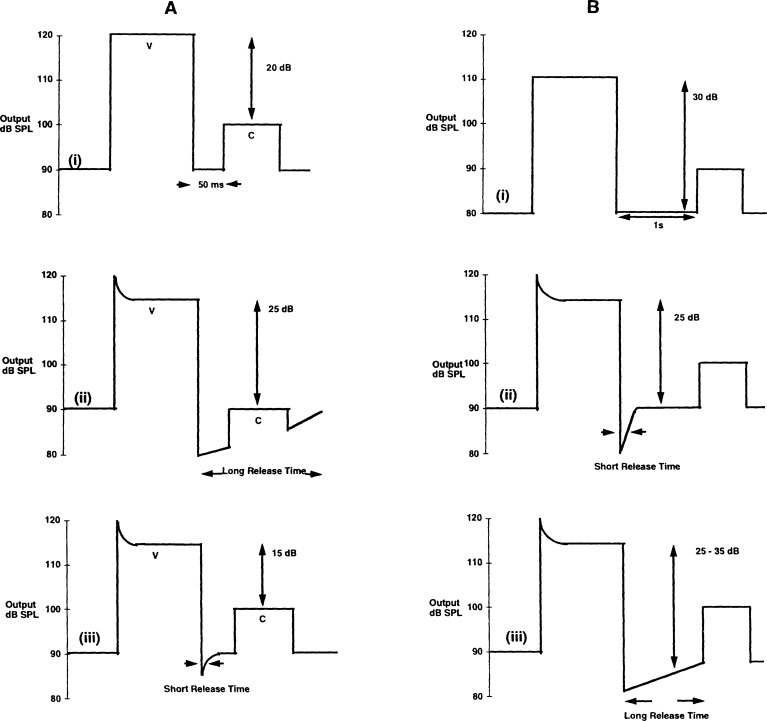
Effect of long and short release times on the output waveform when the input has (A) short intra-syllabic interval, and (B) long inter-syllabic interval. “V” represents vowel and “C” stands for consonant.
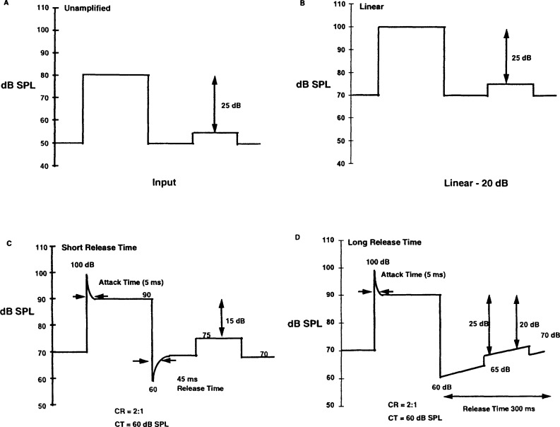
Example to illustrate the reduction in compression ratio from the interaction between release time and inter-syllabic interval. (A) Unamplified signal, (B) linearly amplified signal, (C) short release time, and (D) long release time.
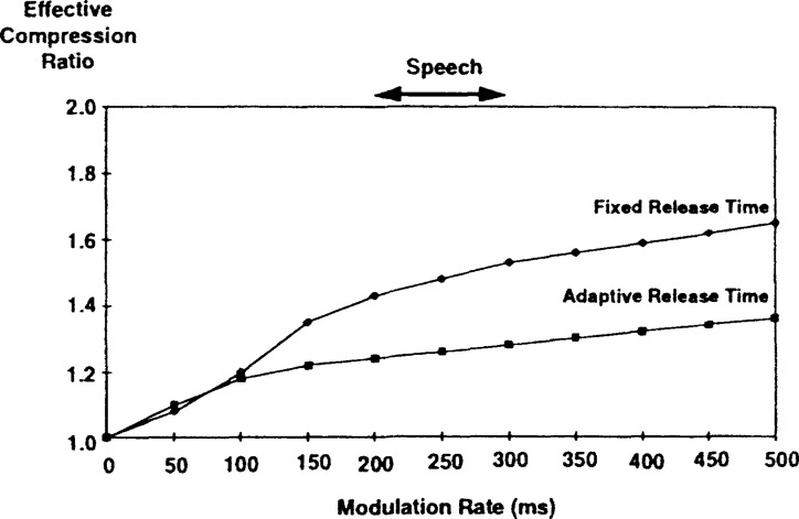
Effective compression ratio of a commercially available compression circuit with fixed release time of 50 ms, and adaptive release time.
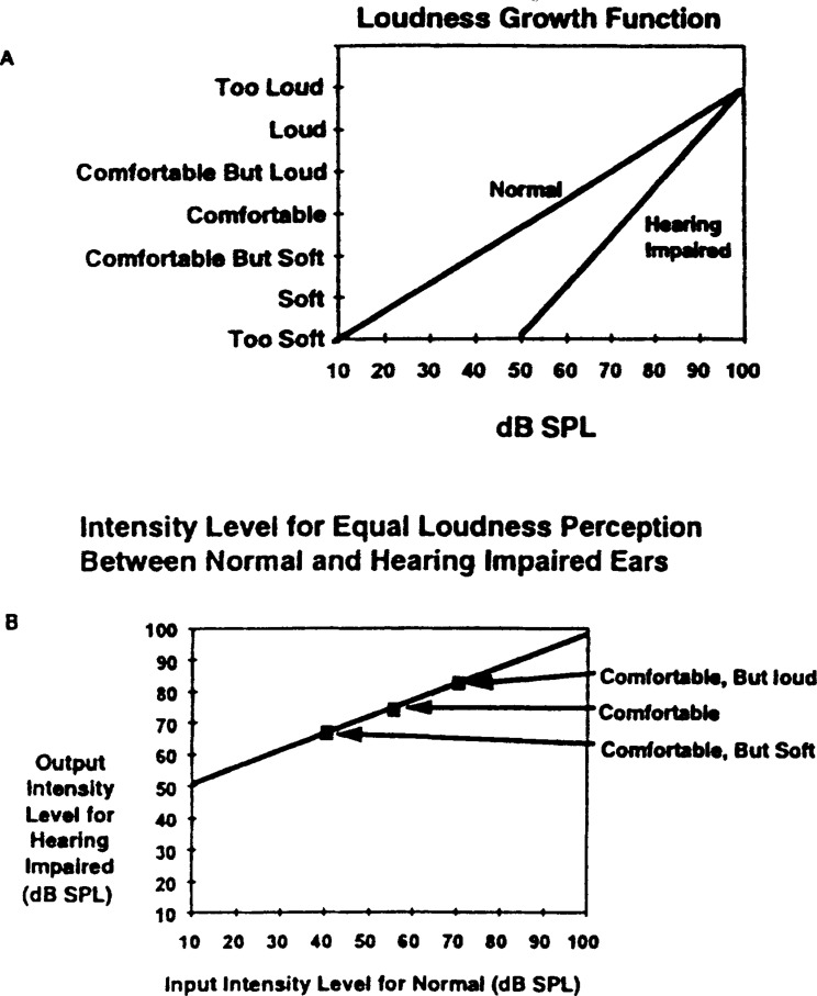
(A) Hypothetical loudness growth function of normal hearing ear and moderately hearing-impaired ear. (B) Output intensity levels for normal hearing and hearing-impaired ears to reach the same loudness perception. The SPL difference between the normal and impaired ears represent the desired gain in the hearing aid to achieve “normal” loudness for the impaired ear.
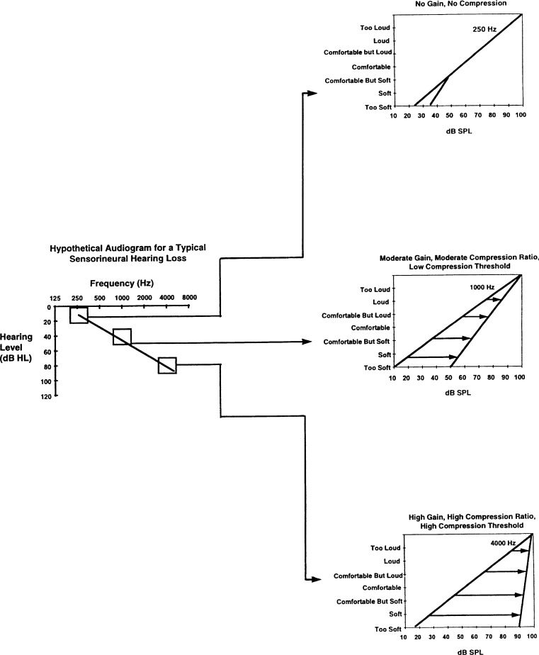
Hypothetical audiogram showing the difference in dynamic range (and thus compression) characteristics across frequencies.
Amount of gain (shown by the length of the arrows) provided by a WDRC (←) and a CL (←) circuit as illustrated on a loudness growth function.
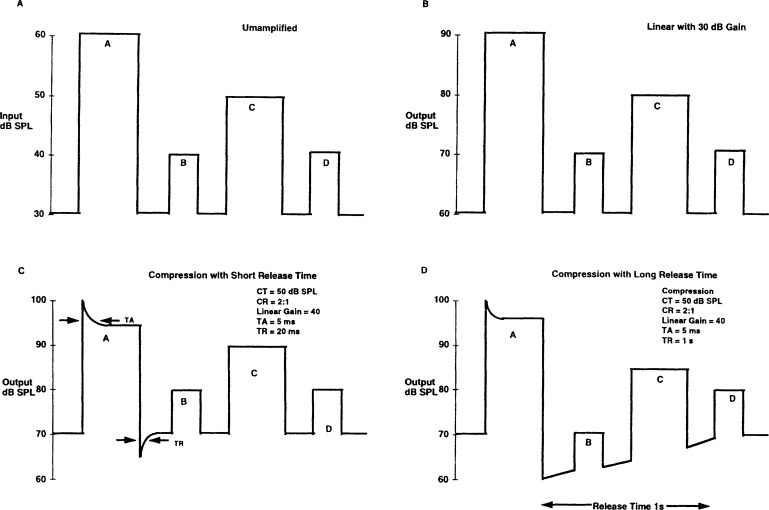
Illustration of how compression can affect the temporal intensity relationship among acoustic segments. (A) No amplification, (B) linear amplification, (C) compression with short release time, and (D) compression with long release time.
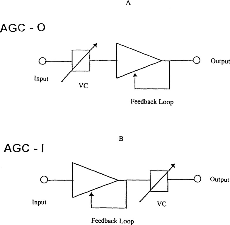
Placement of volume control in a compression circuit: (A) AGC-O, and (B) AGC-I.
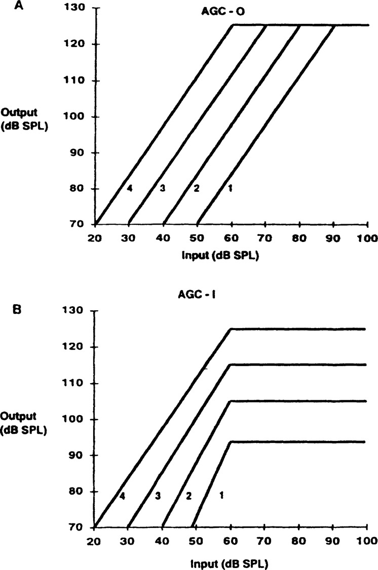
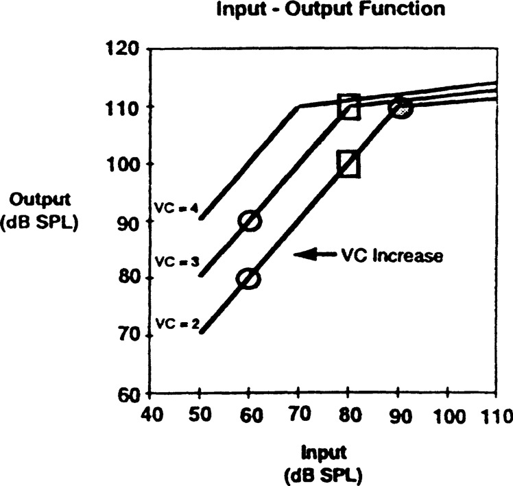
Effect of volume control rotation on the input-output function of an (A) AGC-O hearing aid, and (B) AGC-I hearing aid.
Effect of volume control rotation on the output of an AGC-O hearing aid: Increasing VC leads to an increase in output despite reducing the compression threshold except where saturation is reached.
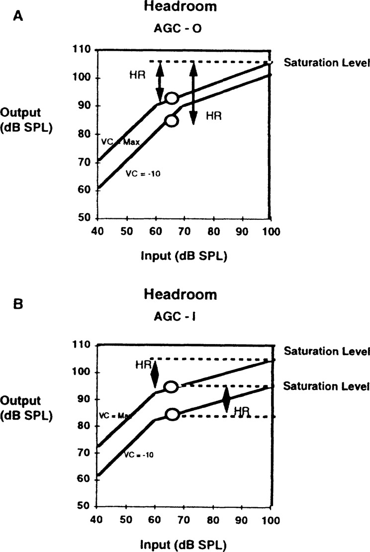
Effect of volume control rotation on the available headroom (HR) in an (A) AGC-O and (B) AGC-I hearing aid.
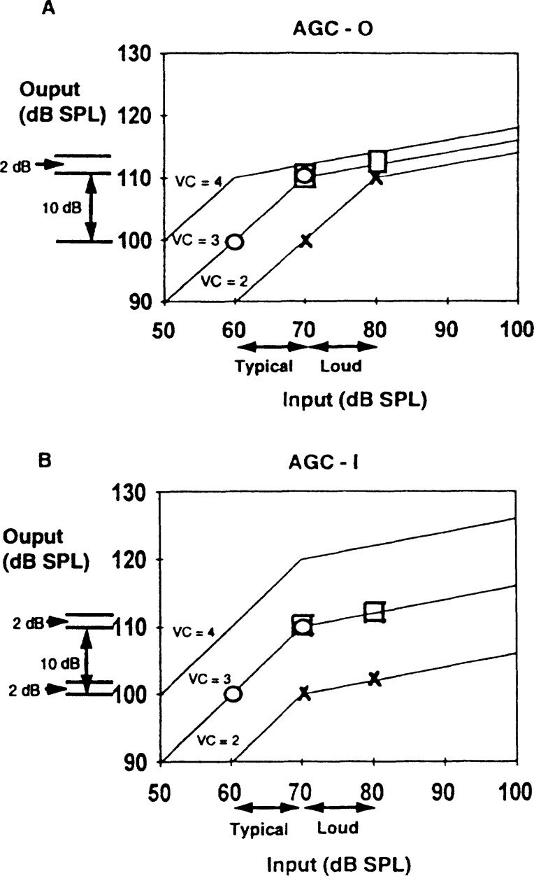
Effect of volume control rotation on the absolute output intensity range in an (A) AGC-O and (B) AGC-I hearing aid. The symbols represent the output level for specific input and VC setting. “O” represents an input from 60 dB SPL to 70 dB SPL and VC = 3. “□” represents an input from 70 dB SPL to 80 dB SPL and VC = 3. “X” represents an input from 70 dB SPL to 80 dB SPL when the volume is turned down to VC = 2.
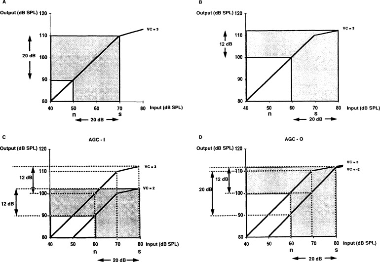
Effect of VC rotation on the long term signal-to-noise ratio. (A) Signal (S) and noise (N) not sufficient to reach the compression threshold. The SNR at the input is preserved. (B) Reduction in output SNR at higher input level. (C) SNR is maintained at a reduced value in an AGC-I hearing aid when the VC is lowered, and (D) SNR at the input is restored in an AGC-O hearing aid with VC reduction.
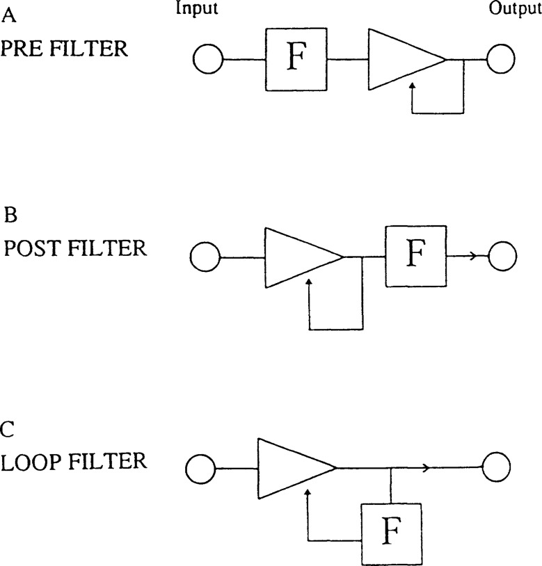
Possible placement of filter within a compression hearing aid: (A) pre-filter, (B) post-filter, and (C) loop filter. “F” represents the filter.
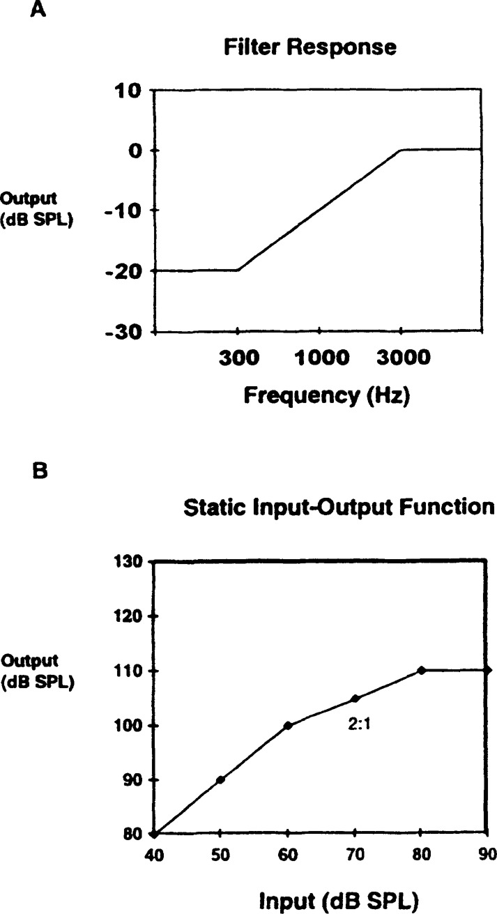
(A) Frequency response of the filter and (B) I-O curve of the compression circuit used in the illustration.
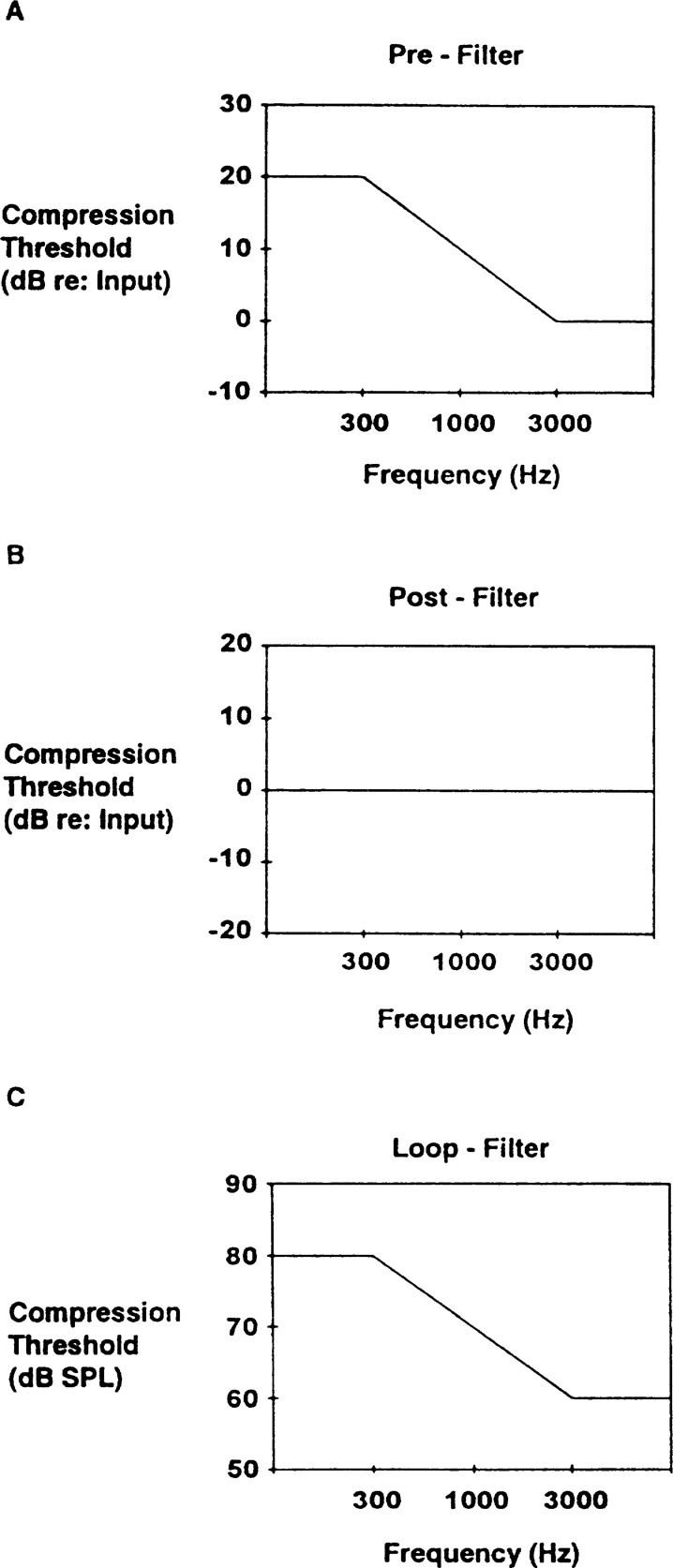
Effect of filter position on compression threshold: (A) pre-filter, (B) post-filter, and (C) loop-filter.
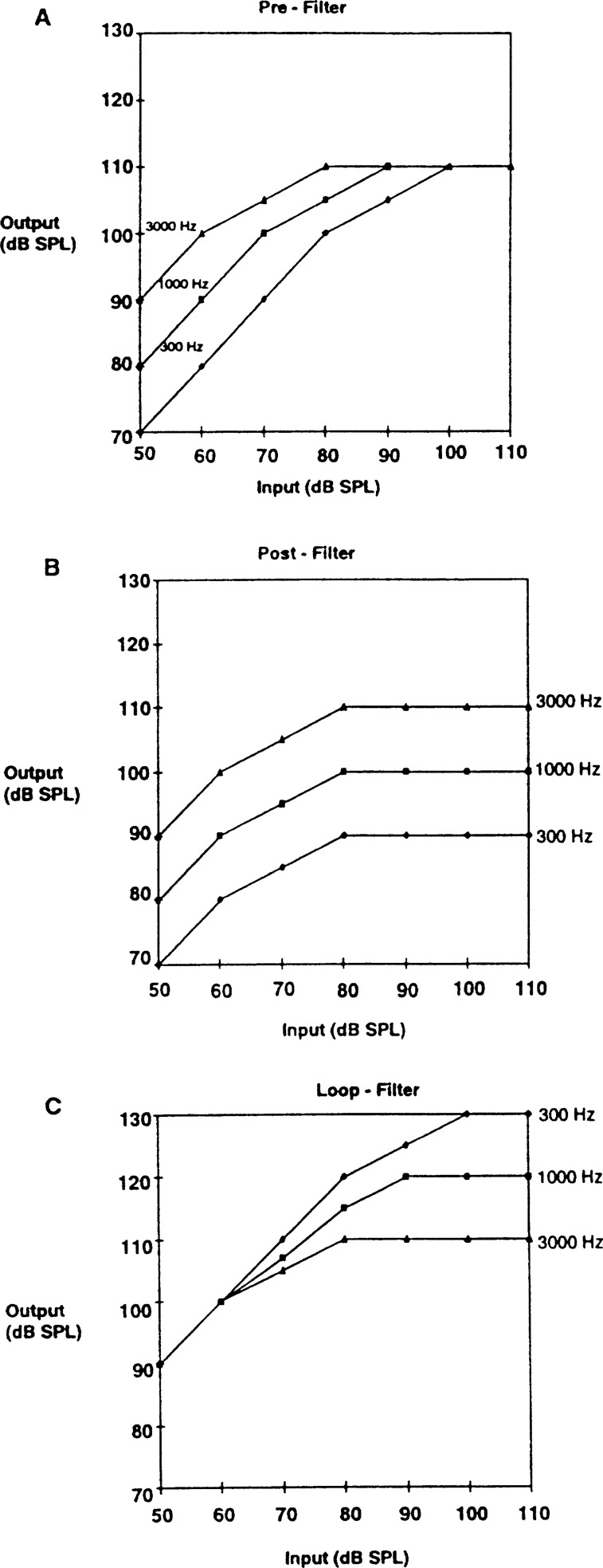
Effect of filter position on input-output curve: (A) pre-filter, (B) post-filter, and (C) loop-filter.
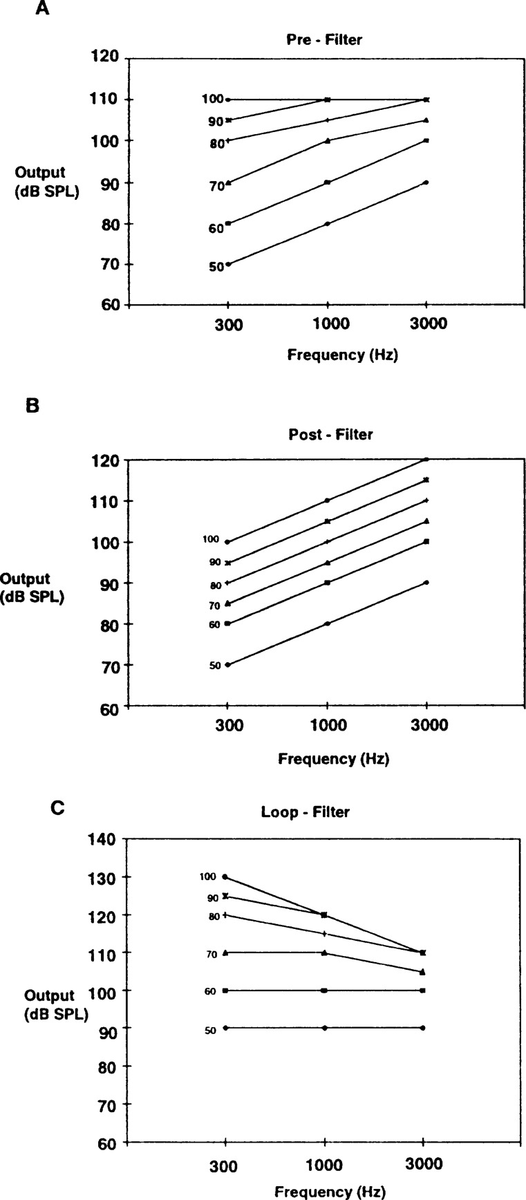
Effect of filter position on frequency response curve at 300 Hz, 1000 Hz, and 3000 Hz: (A) pre-filter, (B) post-filter, and (C) loop-filter. The input levels are indicated as parameter.
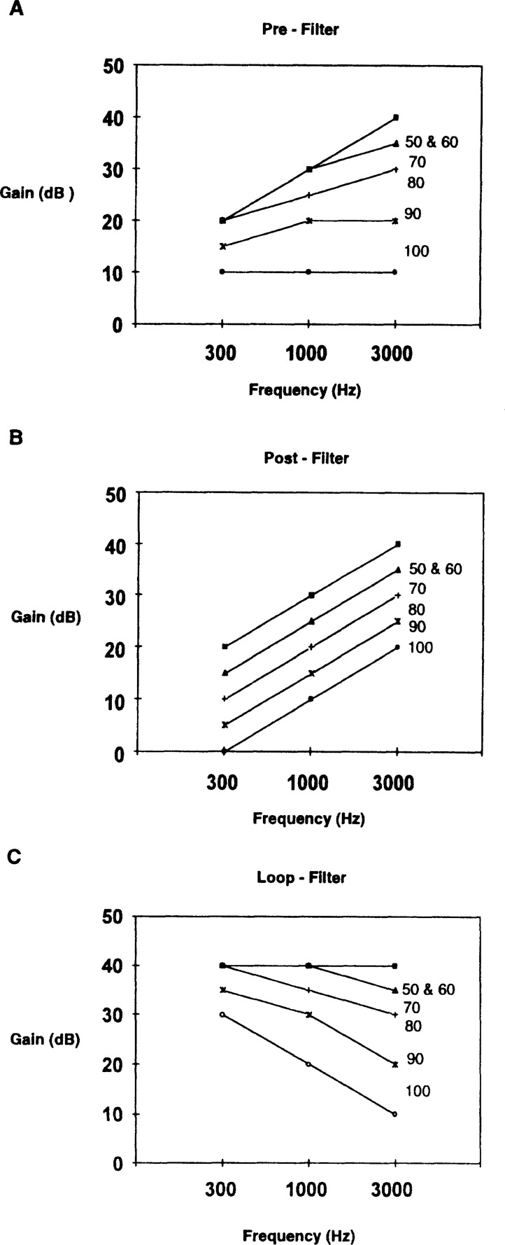
Effect of filter position on frequency-gain curve at 300 Hz, 1000 Hz, and 3000 Hz: (A) pre-filter, (B) post-filter, and (C) loop-filter. The input levels are indicated as parameter.
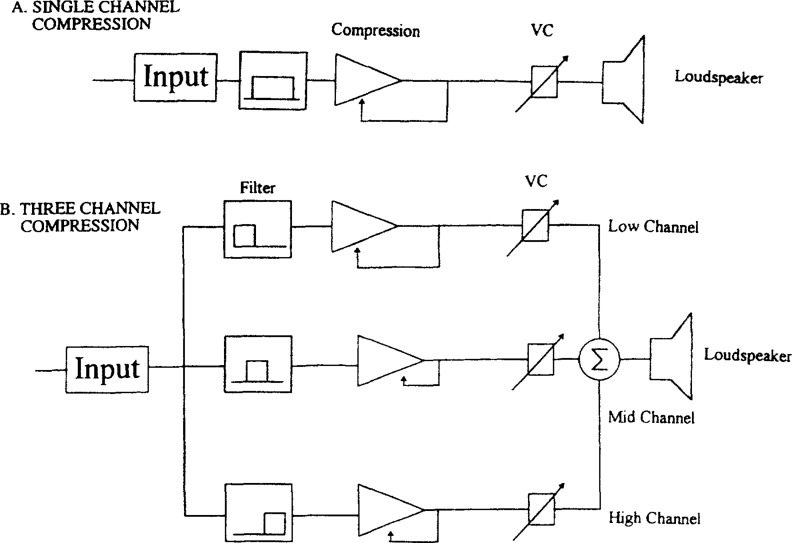
Schematic illustration between a (A) single-channel compression hearing aid, and (B) three-channel compression hearing aid.
Similar articles
-
Clinical experiments with hearing aids with amplitude compression.Scand Audiol Suppl. 1978;(6):293-314. Scand Audiol Suppl. 1978. PMID: 292145
-
Acoustical and Perceptual Comparison of Noise Reduction and Compression in Hearing Aids.J Speech Lang Hear Res. 2015 Aug 1;58(4):1363-76. doi: 10.1044/2015_JSLHR-H-14-0347. J Speech Lang Hear Res. 2015. PMID: 26090648
-
Effects of frequency compression hearing aids for unilaterally implanted children with acoustically amplified residual hearing in the nonimplanted ear.Ear Hear. 2012 Jul-Aug;33(4):e1-e12. doi: 10.1097/AUD.0b013e31824a3b97. Ear Hear. 2012. PMID: 22531574
-
Noise, amplification, and compression: considerations of three main issues in hearing aid design.Ear Hear. 1994 Feb;15(1):2-12. Ear Hear. 1994. PMID: 8194676 Review.
-
Studies with digital hearing aids.Acta Otolaryngol Suppl. 1990;469:57-69. Acta Otolaryngol Suppl. 1990. PMID: 2192534 Review.
Cited by
-
Curriculum for graduate courses in amplification.Trends Amplif. 1998 Mar;3(1):6-44. doi: 10.1177/108471389800300102. Trends Amplif. 1998. PMID: 25425878 Free PMC article. No abstract available.
-
Development of digital hearing AIDS.Trends Amplif. 1997 Jun;2(2):41-77. doi: 10.1177/108471389700200202. Trends Amplif. 1997. PMID: 25425875 Free PMC article. No abstract available.
-
Effects of compression on speech acoustics, intelligibility, and sound quality.Trends Amplif. 2002 Dec;6(4):131-65. doi: 10.1177/108471380200600402. Trends Amplif. 2002. PMID: 25425919 Free PMC article.
-
Selecting and Pre-setting Amplification for Children: Where Do We Begin?Trends Amplif. 1999 Jun;4(2):72-89. doi: 10.1177/108471389900400207. Trends Amplif. 1999. PMID: 25425890 Free PMC article. No abstract available.
-
Frequency-based multi-band adaptive compression for hearing aid application.Proc Meet Acoust. 2019 Dec;39(1):055004. Epub 2020 Jun 22. Proc Meet Acoust. 2019. PMID: 32714483 Free PMC article.
References
-
- Ahren T, Arlinger S, Holmgren S, Jerlvall L, Johansson B, Lindblad A, Persson L, Petterson A, Sjogren H. (1977). Automatic Gain Control in Hearing Aids: The Influence of Different Attack and Release Times on Speech Intelligibility for Hearing Impaired with Recruitment (Report TA 84). Stockholm: Karolinska Institute
-
- Allen J, Jeng P. (1990). Loudness growth in 1/2 octave bands (LGOB): a procedure for the assessment of loudness. J Acoust Soc Amer 88: 745–753 - PubMed
-
- American National Standards Institute. (1987). Specification of Hearing Aid Characteristics. ANSI S3.22–1987. American National Standards Institute, New York
-
- American National Standards Institute. (1992). Testing Hearing Aids with a Broadband Noise Signal. ANSI S3.42–1992.
-
- Baechler H. (1995). Unpublished data.
LinkOut - more resources
Full Text Sources