A framework for modelling gene regulation which accommodates non-equilibrium mechanisms

Abstract

Background: Gene regulation has, for the most part, been quantitatively analysed by assuming that regulatory mechanisms operate at thermodynamic equilibrium. This formalism was originally developed to analyse the binding and unbinding of transcription factors from naked DNA in eubacteria. Although widely used, it has made it difficult to understand the role of energy-dissipating, epigenetic mechanisms, such as DNA methylation, nucleosome remodelling and post-translational modification of histones and co-regulators, which act together with transcription factors to regulate gene expression in eukaryotes.

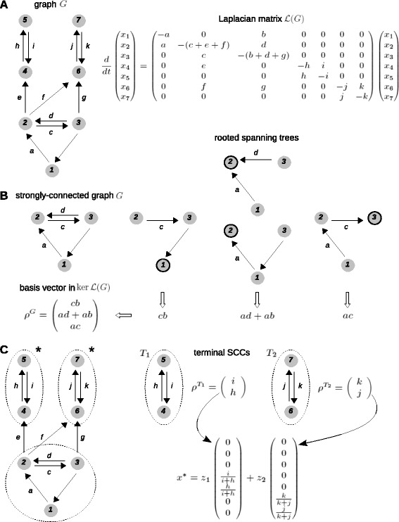
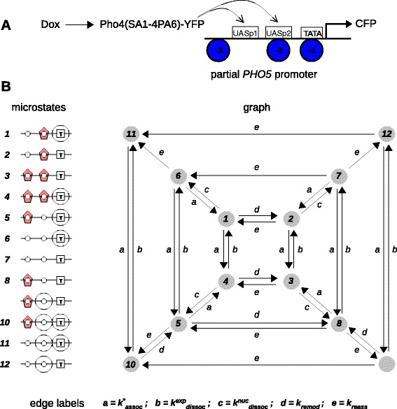
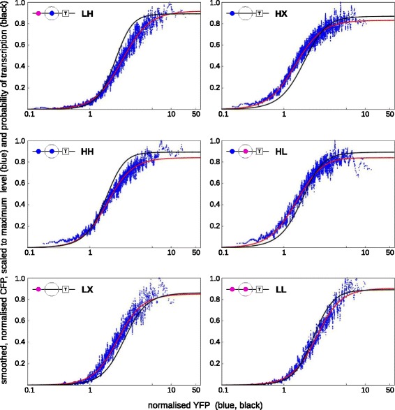
Results: Here, we introduce a graph-based framework that can accommodate non-equilibrium mechanisms. A gene-regulatory system is described as a graph, which specifies the DNA microstates (vertices), the transitions between microstates (edges) and the transition rates (edge labels). The graph yields a stochastic master equation for how microstate probabilities change over time. We show that this framework has broad scope by providing new insights into three very different ad hoc models, of steroid-hormone responsive genes, of inherently bounded chromatin domains and of the yeast PHO5 gene. We find, moreover, surprising complexity in the regulation of PHO5, which has not yet been experimentally explored, and we show that this complexity is an inherent feature of being away from equilibrium. At equilibrium, microstate probabilities do not depend on how a microstate is reached but, away from equilibrium, each path to a microstate can contribute to its steady-state probability. Systems that are far from equilibrium thereby become dependent on history and the resulting complexity is a fundamental challenge. To begin addressing this, we introduce a graph-based concept of independence, which can be applied to sub-systems that are far from equilibrium, and prove that history-dependent complexity can be circumvented when sub-systems operate independently.

Conclusions: As epigenomic data become increasingly available, we anticipate that gene function will come to be represented by graphs, as gene structure has been represented by sequences, and that the methods introduced here will provide a broader foundation for understanding how genes work.

Figure 1

Microstates and graphs. A fragment of a graph is shown (below), with three vertices, i, j and k, and several labelled, directed edges. Vertex i is expanded into a microstate, or snapshot of a DNA state (above), showing some of the features that can be represented (not to scale). Here, a hypothetical promoter region of a gene is shown. Features include sequence-specific transcription factors bound to DNA (grey shapes), additional recruited components, such as transcriptional co-regulators (orange shapes), general-purpose transcriptional machinery, such as Mediator (yellow), general transcription factors (GTFs, blue-green) and RNA Pol II (magenta), along with chromatin remodellers and enzymatic factors that modify the histone tails of nucleosomes (blue shapes). Potential post-translational modifications of transcription factors, co-regulators and histone tails are shown by the corresponding symbols, along with DNA methylation. Distal enhancers may participate through 3D chromatin conformation, such as DNA looping. CTD is the carboxy terminal domain of RNA Pol II. 3D, three dimensional; CTD, carboxy terminal domain; GTF, general transcription factor; Pol, polymerase; Ac, acetylation; Me, methylation; P, phosphorylation; Ub, ubiquitination.

Figure 2

Strongly connected graphs and components. Outlines of hypothetical graphs are shown, omitting some vertices and edges and all labels. (A) A strongly connected graph in which any pair of vertices can be joined, both ways, by a path of contiguous edges in the same direction (central motif). (B) A graph that is not strongly connected can always be decomposed into maximal strongly connected sub-graphs, called strongly connected components (SCCs). The graph shown here has four SCCs demarcated by the dotted lines. In the macroscopic interpretation of one-dimensional chemistry, matter can only flow in one direction between SCCs, so that it eventually accumulates only on the terminal SCCs (marked with an asterisk). In the microscopic interpretation, microstates that are not in a terminal SCC have zero steady-state probability.

Figure 3

Labelled, directed edges for graphs. (A, B) Binding transitions. (C–J) Non-binding transitions. Each example shows a source (left) and a target (right) microstate connected by a labelled edge (curved, barbed arrow). Grey ovals signify background components that make up the microstate. A nominal transcription start site is shown. The magenta shape in (C), (D), (G), (H) and (I) depicts a component of the source microstate that is specifically involved in the reaction represented by the edge. A small dashed arrow signifies an enzymatic action by a component in the source microstate (magenta shape), which remains bound after catalysis. The yellow disc depicts RNA polymerase with a nascent mRNA molecule in the elongating state. The edge-label formula in (B) comes from the rapid equilibrium assumption discussed in the text and is derived in the Methods. 3D, three dimensional; TF, transcription factor; Me, methylation; P, phosphorylation; Ub, ubiquitination.

Figure 4

Calculating microstate probabilities at steady state. (A) On the left, a labelled, directed graph G; on the right, the linear differential equation obtained by taking each edge to be a chemical reaction under mass-action kinetics with the edge label as the rate constant. The resulting matrix is the Laplacian matrix, $\mathcal{ℒ}\left(G\right)$, of G. (B) Illustration of Equation 7. On the left, a strongly connected graph; on the right, the spanning trees of the graph, each rooted at the circled vertex. Because the graph is strongly connected, each vertex has at least one spanning tree rooted there. The basis vector ${\rho }^G\in ker\mathcal{ℒ}\left(G\right)$ is calculated from the spanning trees using Equation 7. Probabilities of microstates are then given by normalising the entries of ρ ^G, as in Equation 4. (C) On the left, the non-strongly connected graph in (A) is shown along with its three strongly connected components (SCCs) demarcated by the dotted lines. The two terminal SCCs are marked with an asterisk and denoted T ₁ and T ₂. Each terminal SCC gives rise to a basis vector in $ker\mathcal{ℒ}\left(G\right)$ using Equation 7, as in (B), and then forming a normalised vector, as shown by following the curved arrows. Note that vertices that are not in a terminal SCC (i.e., vertices 1, 2 and 3) have zero entries in each basis vector. Any steady state, x ^∗, can be expressed as a linear combination of these basis vectors, as in Equation 9 SCC, strongly connected component.

Figure 5

Graph structures satisfying detailed balance. Labels have been omitted for clarity. (A) A sequence of reversible edges, as considered by Ong et al. [46]. (B) A tree of reversible edges. A tree is characterised by having no cycle of reversible edges and is an example of a general graph structure that always satisfies detailed balance, irrespective of the kinds of edges in the graph and the labels on these edges (Methods).

Figure 6

Formation of an inherently bounded chromatin domain [ 47,48 ]. (A) An array of nucleosomes is shown, with nucleation taking place at the right-hand end. White nucleosomes are unmarked, black nucleosomes are marked and grey nucleosomes are either marked or unmarked. Nucleation, at rate k+, is confined to the nucleation site; propagation, also at rate k+, allows a marked nucleosome to propagate the mark to one of its two immediate (unmarked) neighbours; turnover, at rate k_, allows any marked nucleosome, including the nucleation site, to become unmarked. (B) Directed graph for the model with three nucleosomes. Each microstate shows its marking pattern as a bit string with 0 denoting unmarked and 1 denoting marked. The microstates are enumerated by considering the bit string as a number in base 2 notation and adding 1. The edges correspond to nucleation, propagation and turnover, as above. Labels have been omitted for clarity but an edge that increases, respectively decreases, the number of bits has label k+, respectively k_. (C) On the left, an extension of the model to include mark stabilisation, with a stably marked nucleosome shown in magenta. A stabilised mark is no longer subject to turnover. This leads to the non-strongly connected graph shown on the right for an array of two nucleosomes, in which the digit 2 in the microstate description signifies a stabilised mark. Edges that change digit 1 to digit 2 have label k ^∗, while the other edges are labelled as in (B). The strongly connected components (SCCs) are indicated by dotted outlines, with the two terminal SCCs identified by an asterisk.

Figure 7

Regulation of yeast PHO5 , adapted from Figures one and four b of [ 52 ]. (A) Schematic of the experimental set-up. A doxycycline-inducible (Dox), YFP-tagged Pho4, modified to be constitutively active (SA1-4) and constitutively nuclear (PA6), stimulates expression of CFP from a partial PHO5 promoter, with three nucleosomes (-3, -2 and -1) and two Pho4 binding sites, a low-affinity exposed site between nucleosomes -2 and -3 (UASp1) and a high-affinity site occluded by nucleosome -2 (UASp2). The TATA box is occluded by nucleosome -1. (B) The labelled, directed graph of this system, showing the microstates (left) and the labels (bottom), in the notation used by Kim and O’Shea. Label a $\left(k_{\text{assoc}}^{\ast }\right)$ corresponds to Pho4 binding through a Hill function, which arises through the rapid equilibrium mechanism of Figure 3B. Labels b $\left(k_{\text{dissoc}}^{\text{exp}}\right)$ and c $\left(k_{\text{dissoc}}^{\text{nuc}}\right)$ correspond to Pho4 unbinding (Figure 3C) from, respectively, UASp1 and UASp2. Labels d (k _remod) and e (k _reass) correspond to disassembly and assembly, respectively, of nucleosomes (Figure 3F), which introduce the non-equilibrium and irreversible features of the graph. Nucleosome -3 has been ignored in the graph. For other features, see the cited paper CFP, cyan fluorescent protein; YFP, yellow fluorescent protein.

Figure 8

Experimental data and calculated gene-regulation functions of PHO5 variants. Each panel corresponds to one of the six variants, as labelled in the top left with high affinity (H, blue), low affinity (L, magenta) or absent (X), using the microstate schematic from Figure 7B. Each panel shows the smoothed and normalised experimental data for that variant scaled to its maximum expression level (blue points) and plotted as normalised CFP for output against normalised YFP for input, overlaid with calculated gene-regulation functions for that variant (red and black curves), plotted as probability of transcription against normalised YFP, which is assumed to be proportional to Pho4 concentration. The red curves show individual fits to each variant, while the black curves show a collective fit to all variants simultaneously. Further details are provided in the text and the Methods. H, high affinity; L, low affinity; X, absent.

Figure 9

The product graph construction. The corresponding basis vector in the respective Laplacian kernel is shown below each graph. For legibility, the vertices of the product graph are denoted i,j, rather than (i,j). All three graphs are strongly connected. The basis vector for the Laplacian kernel of graph G was calculated in Figure 4B, while that for graph H follows directly from Equation 7. The basis vector for the Laplacian kernel of G×H is given by the Kronecker product formula in Equation 14, as described in the text.

References

1. Ackers GK, Johnson AD, Shea MA. Quantitative model for gene regulation by lambda phage repressor. Proc Nat Acad Sci USA. 1982;79:1129–1133. doi: 10.1073/pnas.79.4.1129. - DOI - PMC - PubMed
1. Buchler N, Gerland U, Hwa T. On schemes of combinatorial transcription logic. Proc Nat Acad Sci USA. 2003;100:5136–5141. doi: 10.1073/pnas.0930314100. - DOI - PMC - PubMed
1. Setty Y, Mayo AE, Surette MG, Alon U. Detailed map of a cis-regulatory input function. Proc Nat Acad Sci USA. 2003;100:7702–7707. doi: 10.1073/pnas.1230759100. - DOI - PMC - PubMed
1. Bintu L, Buchler NE, Garcia GG, Gerland U, Hwa T, Kondev J, Kuhlman T, Phillips R. Transcriptional regulation by the numbers: applications. Curr Opin Gen Dev. 2005;15:125–135. doi: 10.1016/j.gde.2005.02.006. - DOI - PMC - PubMed
1. Vilar JMG, Saiz L. DNA looping in gene regulation: from the assembly of macromolecular complexes to the control of transcriptional noise. Curr Op Genet Dev. 2005;15:136–144. doi: 10.1016/j.gde.2005.02.005. - DOI - PubMed
MeSH terms
LinkOut - more resources