The Multimodal Brain Tumor Image Segmentation Benchmark (BRATS)

Abstract

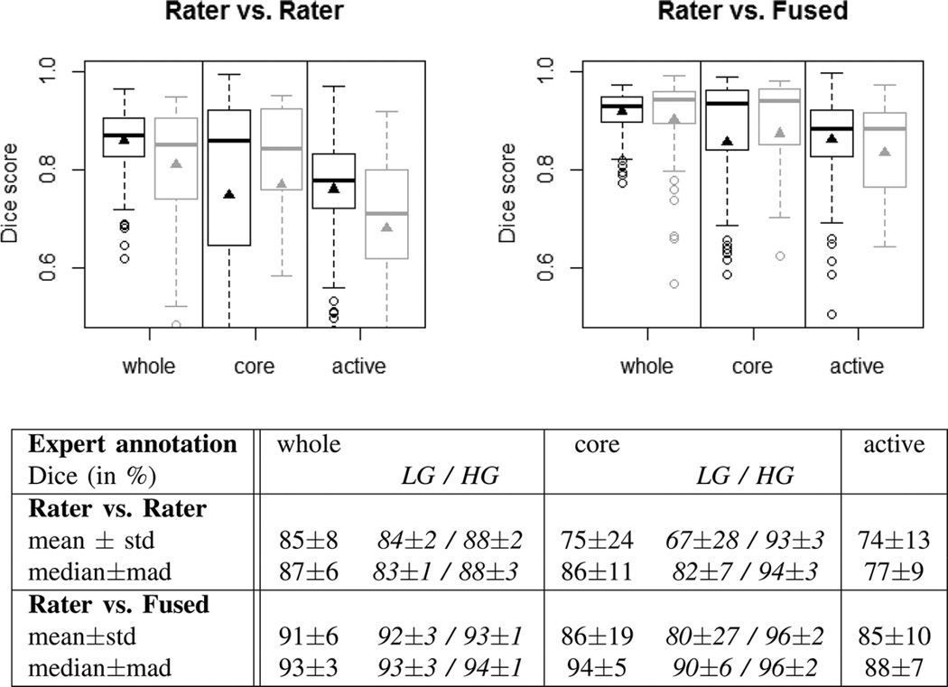
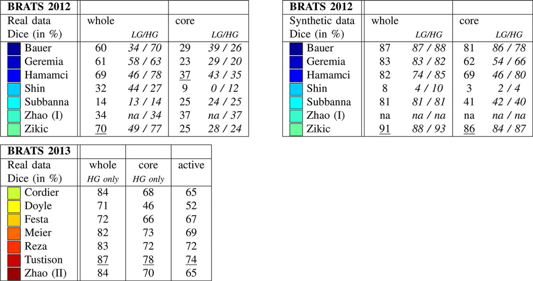
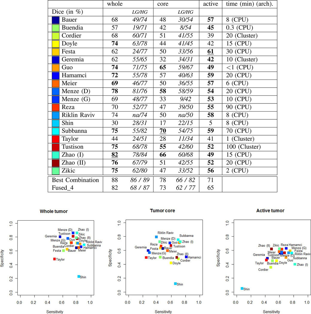
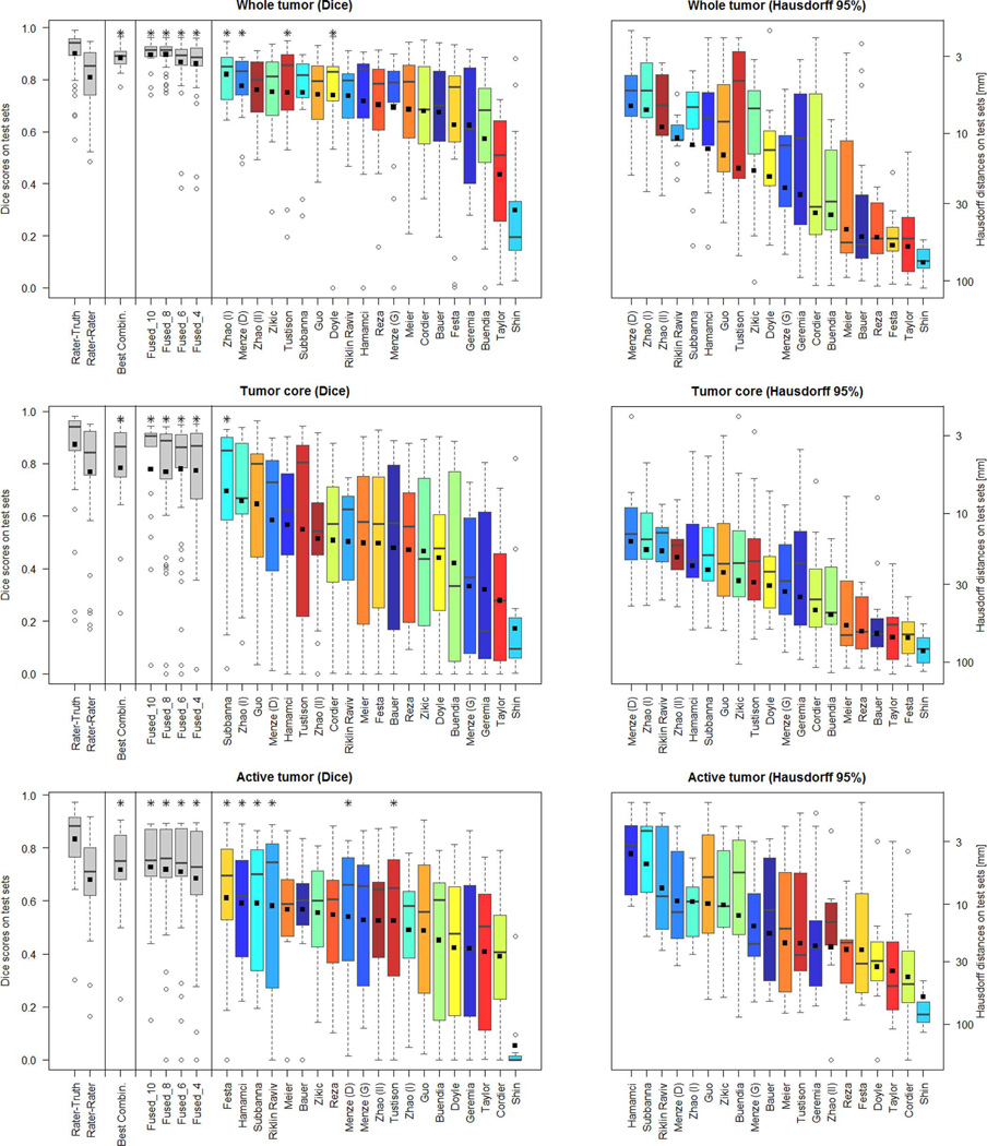
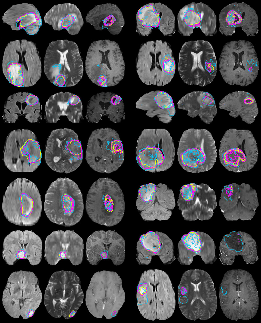
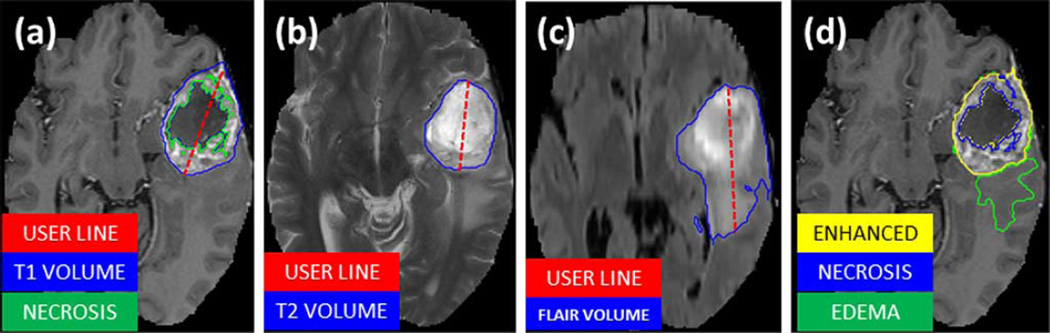
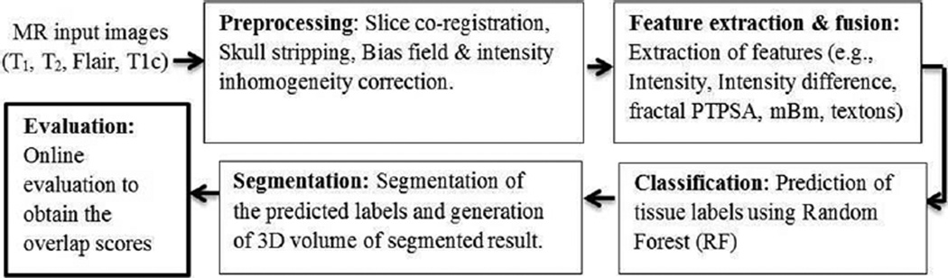
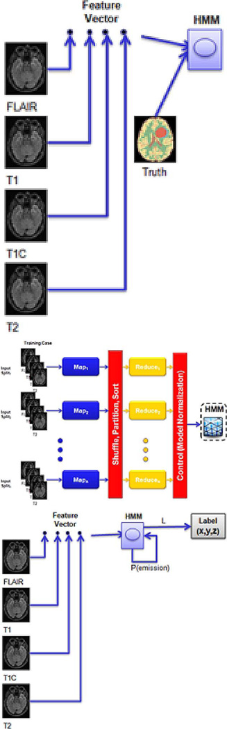
In this paper we report the set-up and results of the Multimodal Brain Tumor Image Segmentation Benchmark (BRATS) organized in conjunction with the MICCAI 2012 and 2013 conferences. Twenty state-of-the-art tumor segmentation algorithms were applied to a set of 65 multi-contrast MR scans of low- and high-grade glioma patients-manually annotated by up to four raters-and to 65 comparable scans generated using tumor image simulation software. Quantitative evaluations revealed considerable disagreement between the human raters in segmenting various tumor sub-regions (Dice scores in the range 74%-85%), illustrating the difficulty of this task. We found that different algorithms worked best for different sub-regions (reaching performance comparable to human inter-rater variability), but that no single algorithm ranked in the top for all sub-regions simultaneously. Fusing several good algorithms using a hierarchical majority vote yielded segmentations that consistently ranked above all individual algorithms, indicating remaining opportunities for further methodological improvements. The BRATS image data and manual annotations continue to be publicly available through an online evaluation system as an ongoing benchmarking resource.

Fig. 1

Results of PubMed searches for brain tumor (glioma) imaging (red), tumor quantification using image segmentation (blue), and automated tumor segmentation (green). While the tumor imaging literature has seen a nearly linear increase over the last 30 years, the number of publications involving tumor segmentation has grown more than linearly since 5–10 years. Around 25% of such publications refer to “automated” tumor segmentation.

Fig. 2

Examples from the BRATS training data, with tumor regions as inferred from the annotations of individual experts (blue lines) and consensus segmentation (magenta lines). Each row shows two cases of high-grade tumor (rows 1–4), low-grade tumor (rows 5–6), or synthetic cases (last row). Images vary between axial, sagittal, and transversal views, showing for each case: FLAIR with outlines of the whole tumor region (left); T2 with outlines of the core region (center); T1c with outlines of the active tumor region if present (right). Best viewed when zooming into the electronic version of the manuscript.

Fig. 3

Manual annotation through expert raters. Shown are image patches with the tumor structures that are annotated in the different modalities (top left) and the final labels for the whole dataset (right). Image patches show from left to right: the whole tumor visible in FLAIR (A), the tumor core visible in T2 (B), the enhancing tumor structures visible in T1c (blue), surrounding the cystic/necrotic components of the core (green) (C). Segmentations are combined to generate the final labels of the tumor structures (D): edema (yellow), non-enhancing solid core (red), necrotic/cystic core (green), enhancing core(blue).

Fig. 4

Regions used for calculating Dice score, sensitivity, specificity, and robust Hausdorff score. Region T₁ is the true lesion area (outline blue), T₀ is the remaining normal area. P₁ is the area that is predicted to be lesion by—for example—an algorithm (outlined red), and P₀ is predicted to be normal. P₁ has some overlap with T₁ in the right lateral part of the lesion, corresponding to the area referred to as P₁ Λ T₁ in the definition of the Dice score (Eq. III.E).

Fig. 5

Dice scores of inter-rater variation (top left), and variation around the “fused” consensus label (top right). Shown are results for the “whole” tumor region (including all four tumor structures), the tumor “core” region (including enhancing, non-enhancing core, and necrotic structures), and the “active” tumor region (that features the T1c enhancing structures). Black boxplots show training data (30 cases); gray boxes show results for the test data (15 cases). Scores for “active” tumor region are calculated for high-grade cases only (15/11 cases). Boxes report quartiles including the median; whiskers and dots indicate outliers (some of which are below 0.5 Dice); and triangles report mean values. Table at the bottom shows quantitative values for the training and test datasets, including scores for low- and high-grade cases (LG/HG) separately; here “std” denotes standard deviation, and “mad” denotes median absolute deviance.

Fig. 6

On-site test results of the 2012 challenge (top left and right) and the 2013 challenge (bottom left), reporting average Dice scores. Test data for 2012 included both real and synthetic images, with a mix of low- and high-grade cases (LG/HG): 11/4 HG/LG cases for the real images and 10/5 HG/LG cases for the synthetic scans. All datasets from the 2012 on-site challenge featured “whole” and “core” region labels only. On-site test set for 2013 consisted of 10 real HG cases with four-class annotations, of which “whole,” “core,” “active” regions were evaluated (see text). Best results for each task are underlined. Top performing algorithms of the on-site challenge were Hamamci, Zikic, and Bauer in 2012; and Tustison, Meier, and Reza in 2013.

Fig. 7

Average Dice scores from the “off-site” test, for all algorithms submitted during BRATS 2012 and 2013. The table at the top reports average Dice scores for “whole” lesion, tumor “core” region, and “active” core region, both for the low-grade (LG) and high-grade (HG) subsets combined and considered separately. Algorithms with the best average Dice score for the given task are underlined; those indicated in bold have a Dice score distribution on the test cases that is similar to the best (see also Fig. 8). “Best Combination” is the upper limit of the individual algorithmic segmentations (see text), “Fused_4” reports exemplary results when pooling results from Subbanna, Zhao (I), Menze (D), and Hamamci (see text). Reported average computation times per case are in minutes; an indication regarding CPU or Cluster based implementation is also provided. Plots at the bottom show the sensitivities and specificities of the corresponding algorithms. Colors encode the corresponding values of the different algorithms; written names have only approximate locations.

Fig. 8

Dispersion of Dice and Hausdorff scores from the “off-site” test for the individual algorithms (color coded), and various fused algorithmic segmentations (gray), shown together with the expert results taken from Fig. 5 (also shown in gray). Boxplots show quartile ranges of the scores on the test datasets; whiskers and dots indicate outliers. Black squares indicate the mean score (for Dice also shown in the table of Fig. 7), which were used here to rank the methods. Also shown are results from four “Fused” algorithmic segmentations (see text for details), and the performance of the “Best Combination” as the upper limit of individual algorithmic performance. Methods with a star on top of the boxplot have Dice scores as high or higher than those from inter-rater variation. Hausdorff distances are reported on a logarithmic scale.

Fig. 9

Examples from the test data set, with consensus expert annotations (yellow) and consensus of four algorithmic labels overlaid (magenta). Blue lines indicate the individual segmentations of four different algorithms (Menze (D), Subbanna, Zhao (I), Hamamci). Each row shows two cases of high-grade tumor (rows 1–5) and low-grade tumor (rows 6–7). Three images are shown for each case: FLAIR (left), T2 (center), and T1c (right). Annotated are outlines of the whole tumor (shown in FLAIR), of the core region (shown in T2), and of active tumor region (shown in T1c, if applicable). Views vary between patients with axial, sagittal and transversal intersections with the tumor center. Note that clinical low-grade cases show image changes that have been interpreted by some of the experts as enhancements in T1c.

Fig. 10

Maximum diameter line drawn by the user to initialize the algorithm for CE-T1 (a), T2 (b), and Flair (c) modalities and the corresponding outputs, for a sample high-grade case. Manual labels overlayed on T1 for a sample slice (d).

Fig. 11

Generic flow diagram of the proposed method.

Fig. 12

Left: Training the HMM model. Center: MapReduce model for HMM-based brain tumor segmentation. Right: Applying the HMM model for segmentation.

References

1. Holland EC. Progenitor cells and glioma formation. Curr. Opin. Neurol. 2001;14:683–688. - PubMed
1. Ohgaki H, Kleihues P. Population-based studies on incidence, survival rates, and genetic alterations in astrocytic and oligodendroglial gliomas. J Neuropathol. Exp. Neurol. 2005 Jun;64(6):479–489. - PubMed
1. Louis DH, Ohgaki H, Wiestler OD, Cavanee WK. WHO classification of tumours of the central nervous system WHO/IARC. Lyon, France: Tech. Rep; 2007. - PMC - PubMed
1. Eisenhauer E, et al. New response evaluation criteria in solid tumours: Revised RECIST guideline (version 1.1) Eur. J. Cancer. 2009;45(2):228–247. - PubMed
1. Wen PY, et al. Updated response assessment criteria for high-grade gliomas: Response assessment in neuro-oncology working group. J Clin. Oncol. 2010;28:1963–1972. - PubMed
Publication types