Detecting causality from nonlinear dynamics with short-term time series

Abstract

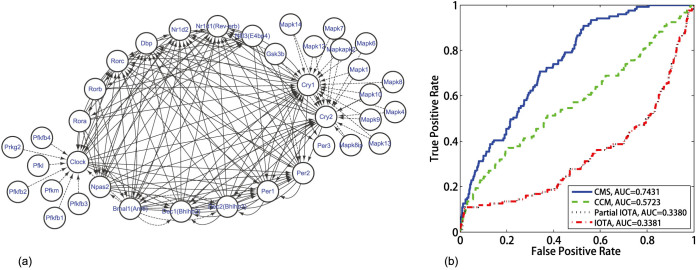
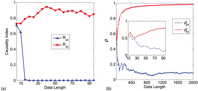
Quantifying causality between variables from observed time series data is of great importance in various disciplines but also a challenging task, especially when the observed data are short. Unlike the conventional methods, we find it possible to detect causality only with very short time series data, based on embedding theory of an attractor for nonlinear dynamics. Specifically, we first show that measuring the smoothness of a cross map between two observed variables can be used to detect a causal relation. Then, we provide a very effective algorithm to computationally evaluate the smoothness of the cross map, or "Cross Map Smoothness" (CMS), and thus to infer the causality, which can achieve high accuracy even with very short time series data. Analysis of both mathematical models from various benchmarks and real data from biological systems validates our method.

Figure 1. Illustration of mutual neighbors, cross map and smoothness.

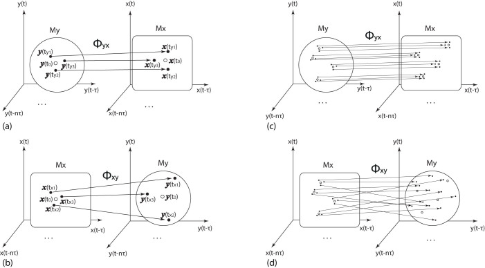
(a) For one point y(t₀) ∈ M_y and its counterpart x(t₀) ∈ M_x, one can find the nearest neighbors , , for y(t₀) and define the mutual neighbors , , for x(t₀). The map between the nearest neighbors and mutual neighbors is defined as cross map Φ_yx. In the case x causally influences y, the cross map Φ_yx maps a neighborhood to a neighborhood. (b) In the case y does not causally influence x, the cross map Φ_xy does not necessarily map a neighborhood to a neighborhood. (c) and (d) The global smoothness of Φ_yx and Φ_xy built from local smoothness.

Figure 2. Illustration for the time series length and convergence of nearest neighbors.

Here the time series are generated by one chaotic Lotka-Volterra system. (a) A reconstructed attractor from time series of 7000 samples, and the 5 nearest neighbors (5NN) of one center point. (b) A reconstructed attractor from time series of only 100 sampled points and the 5 nearest neighbors of the same center point. Inset: the comparison of the 5 nearest neighbors for both (a) and (b), where the latter set of points are apparently not close to the center point at all.

Figure 3. Sketch of the cross map smoothness learned by a neural network (NN).

(a) and (b) Illustrations for the neural network's approximation ability for smooth map and unsmooth map. Here the map surface in (a) is assumed to be x = y₁ + y₂ and the surface in (b) is simply generated by random points. (c) and (d) The prediction error (or the smoothness of Φ) for cases in (a) and (b) respectively, where the leave-one-out scheme is used to calculate errors. (e) Assume that x causally influences y, the information of x has been encoded in M_y and consequently Φ: M_y → M_x maps a neighborhood of y to a neighborhood of x, implying Φ_yx is smooth. 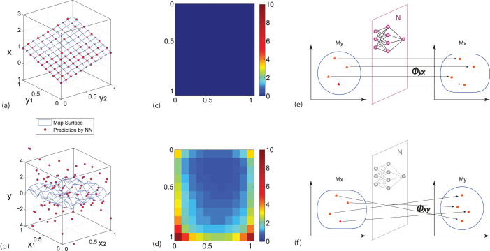Thus a neural network can be trained to approximate the map based on the measured data on M_x and M_y. (f) Assume that y has no impact on x, then M_x has no information from y. Training a neural network to approximate the unsmooth map Φ: M_x → M_y will fail.

Figure 4. Coupling relationship patterns (coupling strength γ in the left column) and the corresponding causality patterns (detected index R in the right column), where only the significantly detected causal relations above threshold are shown.

(a) Unidirectional causality pattern in the 2 species model. (b) Bidirectional causality pattern in the 2 species model. (c) Fan-out causality pattern. (d) Fan-in causality pattern.

Figure 5. Causality index detected for varying the coupling strength values.

Dotted lines are the fitted trend curves. (a) Unidirectional case. (b) Bidirectional case.

Figure 6. Causality detection for a parameter-varying system in a piecewise manner.

The dashed square waves represent the random switching of the coupling parameters between zero and nonzero values, and the solid lines represent the detected strengths of causative effectiveness over each time window.

Figure 7

(a) Regulatory network with the selected 50 genes of E. coli. (b) The ROC curves of the detection results by our method (CMS), with different levels of the noise condition.

Figure 8

(a) Regulatory network with the selected 100 genes of S.cerevisiae. (b) Regulatory network with the selected 150 genes of S.cerevisiae. (c) The ROC curves of the results for the network in (a) by our method, with different levels of the noise condition. (d) The ROC curves of the results for the network in (b) by our method, with different levels of the noise condition.

Figure 9

(a) Regulatory network with the selected circadian genes, where the solid lines indicate gene-level regulations and the dashed lines imply protein-level interactions. (b) The ROC curves of the results, with four methods tested on the same data set.

Figure 10

(a) The causality detected by CMS based on different lengths of time series. (b) The causality detected by CCM based on different lengths of time series, where the inset is the enlarged part for the same data length as in (a).

Figure 11. Comparison results for three methods on theoretical models.

The left column shows the causality patterns in 5 models, where black blocks shows causality from vertical variables to horizonal variables. The gray scale represents the strength of the detected causality between 0 (white) and 1 (black).

References

-
- Granger C. W. J. Investigating causal relations by econometric models and cross-spectral methods. Econometrica 37, 424–438 (1969).
- Sugihara G. et al. Detecting causality in complex ecosystems. Science 338, 496–500 (2012). - PubMed
- Haufe S., Nikulin V. V., Mller K.-R. & Nolte G. A critical assessment of connectivity measures for EEG data: A simulation study. NeuroImage 64, 120–133 (2013). - PubMed
- Schreiber T. Measuring information transfer. Phys. Rev. Lett. 85, 461 (2000). - PubMed
- Paluš M., Komárek V., Hrnčíř Z. & Štěrbová K. Synchronization as adjustment of information rates: detection from bivariate time series. Phys. Rev. E 63, 046211 (2001). - PubMed
Publication types
MeSH terms
Substances
LinkOut - more resources
Full Text Sources
Other Literature Sources